Quantum Field Theory

The Field Equation
Quantization
Green's Function and Renormalization
Perturbation Theory and S Matrix
Feynman Diagram
Quantum Electrodynamics (QED)
A Very Brief Overview of the Standard Model

The Field Equation

Quantum Field Theory can be considered as "field + quantization". Followings is a mathematical formulation (at 2nd year undergraduate level) on the construction of quantum field and its application to elementary particle physics.

The dynamic of the field is determined by the field equation. The field equation for the neutral scalar meson field is a very simple kind of Klein-Gordon Equation as shown below:

---------- (1)

where m is a parameter related to the mass, is the field, which is a complex function (with real and imaginary parts) of x, y, z, and t (simply represented by x in the equation),
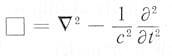, and

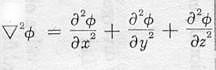
are the Laplacians in four dimensional space-time and three dimensional space respectively. The wave equations and many systems in physics and engineering are constructed with these Laplacian operators.

The field can be expressed in a series expansion in terms of the harmonic functions and the coefficients c_k's, where k is a four dimensional vector related to the momentum and energy of the particle:

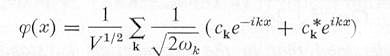---------- (2)

which is just a Fourier Series where the coefficients are to be determined by the field:

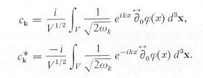---------- (3)

Quantization

Quantization of the field is accomplished by demanding the coefficients c_k's to satisfy the following commutation rules:

---------- (4)

If a number operator N_k = c_k*c_k is defined such that it operates on the state vector |n_k> to generate:
N_k|n_k> = n_k|n_k>
where n_k is the number of particles in the k state; it can be shown that
c_k*|n_k> = (n_k+1)^1/2|n_k+1>
c_k|n_k> = n_k^1/2|n_k-1>
Thus c_k* increases the number of particles in the k state by 1, while c_k reduces the number of particles in the k state by 1. They are called creation and annihilation operator respectively. The complete set of eigenvectors is given by:

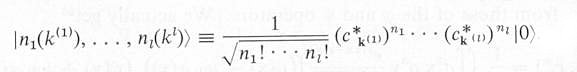---------- (5)

for all values of k^l and n_l. They form an abstract space called the Hilbert space with all the eigenvectors orthogonal (perpendicular) to each others and the norm (length) equal to 1.

In particular, the vacuum state is:

---------- (6)

which corresponds to no particle in any state - the vacuum.

Green's Function and Renormalization

The above treatment is for the case of free field. The mathematics becomes more complicated when there is interaction with the field. The simplest case is to include the source of the field in the free field equation. An additional term is inserted to the right of Eq.(1) :

---------- (7)

where the label "o" designates quantities associated with the "bare field".

Invoking the Green's function technique, the solution of this equation is given by:

---------- (8)

where the first term is the free field solution and the Green's function inside the integral is the solution of the equation with a point source at point y in the general form:

---------- (9)

where the delta function on the right hand side equals to 1 for x = y, and 0 otherwise.

It can be shown that the "bare field" can be expressed in terms of c_k's similar to the case of the free field, but these coefficients are now modified by an additional term related to the structure of the source. As a result the norm (length) of the eigenvectors are no longer equal to 1. To recover this definition, they have to be "renormalized" by the renormalization constant Z^1/2, which has the values in general; it is equal to 1 for free field and 0 for a point source. The renormalized field, mass, and energy are and E_n^R = Z^-1E_n^o respectively. The physical mass m_R is the experimentally observed mass, m_o is an unspecified parameter (called "bare mass") which together with Z^-1 determine a value in agreement with experiment. In a realistic, fully quantized system, perturbation theory must be used to obtain any numerical result. However, it is found that perturbation theory calculations always lead to an infinity value for Z so that the ''bare" quantities such as m_o would also be infinity to yield a finite value for m_R.

Perturbation Theory and S Matrix

It is not possible to obtain an analytical solution for the field equation with the field itself in the interaction term. A perturbation theory was developed to obtain approximate solutions step by step. The interaction between a charged fermion and the photon is in the form , where A is the electromagnetic vector potential and is the field for the fermion, which appears on both side of the Green's function solution as shown in Eq.(8). An iteration procedure yields a sum of integrals as shown in the formula below:

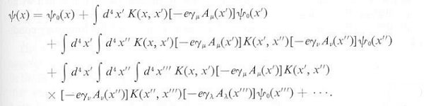---------- (10)

where K is the Green's function. In this form the unknown field on the left hand side is now expressed in terms of all known quantities on the right hand side. The first term is the free field solution, and the integration is over all the space-time x^', x^'', x^''', ... Note that each of the following term is multiplied by the power of e, from e¹, to e², ... Since e=1/137 for the electromagnetic interaction, computation on a few terms would be sufficient to obtain a result with acceptable accuracy.

Another formulism is the S-matrix theory, which was very popular many years ago. It is the transition probability expressed in an expansion as the result of the iteration procedure on the transition operator, which transforms the system from an initial state (at time negative infinity) to a final state (at time positive infinity) as shown in the formula below.

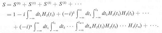---------- (11)

where H_I involves the interaction fields (integrating over all space and multiplied by the coupling strength) and
t₁ > t₂ > ... > t_n-1. In this picture the fields obey the free field equations, the interaction enters via H_I. It was thought that since we cannot measure the fields directly, so we should not talk about it, while we do measure S-matrix elements, so this is what we should be mindful about. It is now realized that analyzing the S-matrix alone is not sufficient, information on the quantum fields is also necessary. It can be shown that the various orders in the S-matrix are related to the petrubation expansion in Eq.(10).

Let us take the nucleon-pion system as an example of S-matrix application:

---------- (12)
---------- (13)

where Eq.(12) is the free field equation for the pion, and Eq.(13) is the free field equation for the nucleon (the Dirac equation). Expressing in terms of the field itself, it can be shown that the quantization rules in Eq.(4) become:

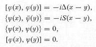---------- (14)

where {a,b} = ab + ba is the anticommunition expression, and the quantities on the right-hand side are the Green's functions for the pion and nucleon respectively. Since the interaction is g_o the nth order term in the S-matrix expansion Eq.(11) has the explicit form:

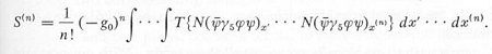---------- (15)

where the symbol N is the normal-order operator, which shifts all the creation operators to the left (to avoid infinite vacuum energy), while T is the time-order operator, which re-arranges the fields so that the one associated with later time is on the left (to take care of the integration limits in Eq.(11)).

Feynman Diagram

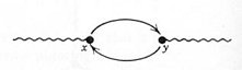
The first order term is:

---------- (16)

The mathematical entities inside the integral can be represented graphically by the following conventions:

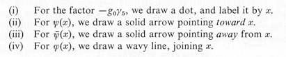
which translates S⁽¹⁾ into a graph called the Feynman diagram:

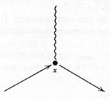
It represents the process of the annihilation of a pair of nucleon and anti-nucleon and the creation of a pion.
In the next higher order term the normal operator will sometimes produces a Green's function such as . This is usually referred to as propagator and graphically represented by a wavy line running from x to y as show below:

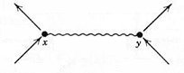
which corresponds to the scattering of two nucleons by exchanging a pion. Another graph such as the one below:

represents the process of virtual pair creation and annihilation - the vacuum fluctuation.

The Feynman rules are summarized in the table below:

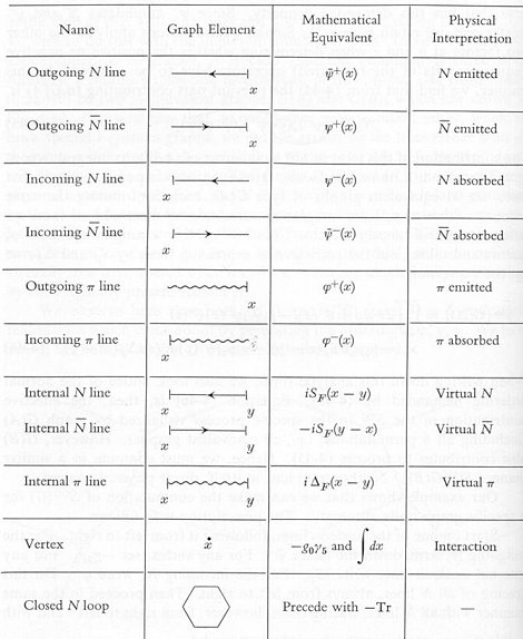
where the + and - superscripts refer to the positive frequency (e^ikx) and negative frequency (e^-ikx) expansion in Eq.(2), N represents the nucleon and represents the anti-nucleon.

Feynman diagrams can be divided into two types, "trees" and "loops", on the basis of their topology. Tree diagrams have no loops; that is, they only have branches. They describe process such as scattering, which yields finite result and reproduces the classical value. Loop diagrams, as their name suggests, have closed loops in them such as the one for vacuum fluctuation. The process in "loops" diagrams involves virtual particles and is usually divergent (becomes infinity at some limits). The infinities are removed by the renormalization precedure similar to the mass renormalization mentioned earlier. Virtual particles can appear and disappear violating the rules of energy and momentum conservation as long as the uncertainty principle is satisfied. They are said to be "off mass-shell", because they do not satisfy the relationship E² = p²c² + m²c⁴.

Quantum Electrodynamics (QED)

Quantum electrodynamics, or QED, is a quantum theory of the interactions of charged particles with the electromagnetic field. It describes mathematically not only all interactions of light with matter but also those of charged particles with one another. QED is a relativistic theory in that Albert Einstein's theory of special relativity is built into each of its equations. That is, the equations are invariant under a transformation of space-time. The QED theory was refined and fully developed in the late 1940s by Richard P. Feynman, Julian S. Schwinger, and Shin'ichiro Tomonaga, independently of one another. Because the behavior of atoms and molecules is primarily electromagnetic in nature, all of atomic physics can be considered a test laboratory for the theory. Agreement of very high accuracy makes QED one of the most successful physical theories so far devised.

The formulism for QED is very similar to the nucleon-pion system in Eqs.(12) and (13). While Eq.(13) for fermion is readily applicable (with appropriate value for k_o, which is proportional to the mass of the fermion); Eq.(12) is replaced by the Maxwell equations:

where E, B are the electric and magnetic field respectively, j is the current density, rho is the charge density, and c is the velocity of light.

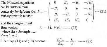
By virtue of the antisymmetry of Eq.(21), the continuity equation for the charge-current density is automatically satisfied, i.e.,

The vector potential is introduced by:

---------- (24)

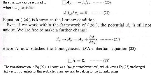
This definition is used for simplifying computations. It incorporates Eqs.(19) and (20) into the formulism automatically. There is arbitrariness when the Maxwell equations are written in this form. By imposing particular conditions to the arbitrariness,

The vector potential A can always be decomposed into a transverse component and a longitudinal component (with respect to the direction of motion) as shown in Eq.(29) such that Eqs.(30) and (31) are satisfied:

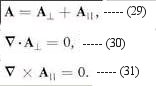
It can be shown that the longitudinal component and A_o together give rise to the instantaneous static Coulomb interactions between charged particles, whereas the transverse component accounts for the electromagnetic radiation of moving charged particles. The transverse electromagnetic fields provides a simple and physically transparent descriptions of a veaiety of processes in which real photons are emitted, absorbed, or scattered. The three basic equations for the free-field case are:

where A satisfies the transversality condition in Eq.(30).

Eq.(33) is in a form very similar to the Klein-Gordon Equation Eq.(1) or Eq.(12) except that the mass term vanishes (because the photon has no rest mass) and the field is a vector (instead of scalar) with two transverse components (polarization) perpendicular to each other. Thus A can be expressed in Fourier series similar to Eq.(2):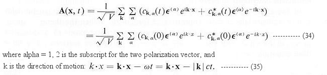
The quantization rules for the electromagnetic field is very similar to that in Eq.(4):

---------- (36)

where the a_k's are related to the c_k's by:

---------- (37)

Construction of the eigenvectors follows exactly the same way as in Eqs.(5) and (6) with an additional index for polarization.

Interaction between photon and fermion, e.g., electron can be introduced by demanding local gauge invariance for the formulism. With this constraint on the quantum field theory, the ordinary derivative in Eq.(13) becomes the covariant derivative:

and the interaction takes the form:

where e is the coupling constant. (See appendix on "Abelion/non-Abelion Groups and U(1), SU(2), SU(3)" for a discussion about the concept of gauge or phase transformation.)

The photon-electron processes are described by substituting Eq.(39) to H_I in the S matrix expansion Eq.(15):

The first order processes -

where the electron field has been decomposed to:

and the symbol X may stand for an interaction with an external classical potential, the emission of a photon, or the absorption of a photon. The realization of a particular process depends entirely on the initial and final states.
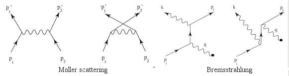
The second order processes -
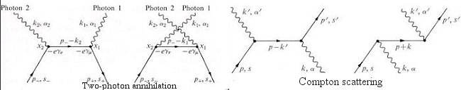
- Two-photon annihilation - Pair of an electron and positron into two gamma rays.
- Compton scattering - It occurs when an electron and a photon collide and scatter elastically.
- Moller scattering - It is the scattering of two relativistic electrons.
- Bremsstrahlung - It is the process by which radiation is emitted from an electron as it moves past a nucleus.
Higher order processes -
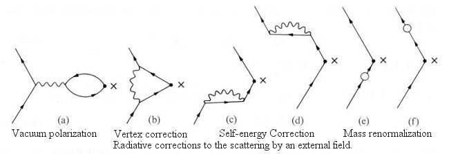
- Vacuum polarization - It produces a correction to the coupling constant (electric charge) and contributes to the Lamb shift, which is a small splitting of hydrogen atom energy levels caused by the interaction with the virtual pair (of electron and positron).
- Vertex correction - A correction to the electron vertex function, which contributes to the anomalous electron magnetic moment.
- Self-energy - The interaction of a charged particle with its own field and it usually gives rise to infinite self-energy and infinite mass.
- Mass renormalization - The observed mass is generated by combining the bare mass and the (calculated) divergent mass.

In summary QED rests on the idea that charged particles (e.g., electrons and positrons) interact by emitting and absorbing photons, the particles of light that transmit electromagnetic forces. These photons are virtual; that is, they cannot be seen or detected in any way because their existence violates the conservation of energy and momentum. The particle exchange is manifested as the "force" of the interaction, because the interacting particles change their speed and direction of travel as they release or absorb the energy of a photon. Photons also can be emitted in a free state, in which case they may be observed. The interaction of two charged particles occurs in a series of processes of increasing complexity. In the simplest, only one virtual photon is involved; in a second-order process, there are two; and so forth. The processes correspond to all the possible ways in which the particles can interact by the exchange of virtual photons, and each of them can be represented graphically by means of the Feynman diagrams. Besides furnishing an intuitive picture of the process being considered, this type of diagram prescribes precisely how to calculate the observable quantity involved.

A Very Brief Overview of the Standard Model

It is beyond the scope of this webpage to present a comprehensive review of the Standard Model. The following is a crude attempt to provide a glance of the subject matter by introducing the Lagrangian density _{Standard Model} for the Standard Model. The field equations are derived by minimizing the "Action'' , which is related to the Lagrangian density. Thus instead of writing down the field equations explicitly such as in Eqs.(17) - (20) or Eqs.(13) and (38), the dynamics of the electro-weak interaction can be expressed in term of the Lagrangian density:

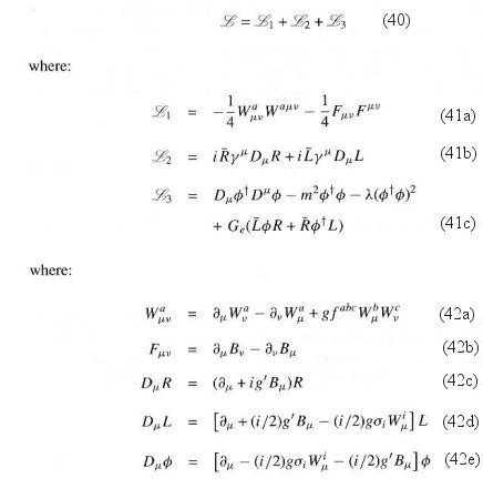
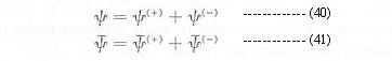
This is known as the Weinberg-Salam Model. The lepton Lagrangina density in Eq.(40) consists of three parts. ₁ is the gauge bosons part; ₂ is the fermionic part; and ₃ is the scalar Higgs sector, which generates mass for the gauge bosons and the fermions.

Meaning of the symbols in the Lagrangina density :

The symbols and are indices for the space-time components running from 1 to 4. Whenever an index appears in both the subscript and superscript, it signifies a summation over these components.
W^a is related to the three gauge (vector) bosons with the index "a" running from 1 to 3.
F is the anti-symmetric tensor for the electromagnetic field as shown in Eq.(24), where the vector potential A is now denoted by B.
f^abc is the antisymmetric tensor such that f¹²³ = +1, f²¹³ = -1, f¹¹³ = 0, ... etc.
Since there is no right-handed neutrino in nature, the fermionic field consists of a left-handed isodoublet and a right-handed isosinglet as shown below -

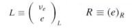
---------- (42f)

This curious feature, that the electron is split into two parts is a consequence of the fact that the weak interactions violate parity and are mediated by V - A interactions, where V stands for vector and A stands for axial vector (also known as pseudovector, which changes sign under a parity transformation). The axial vector interaction is hidden in the last term of Eq.(42d). The asymmetric forms for the fermion fields in Eq.(42f) is a way to portrait the chiral nature of the objects in weak interaction - the left-handed version is different from the right-handed one. Note that in Eq.(42c) the right-handed field R does not participate in the weak interaction involving the vector bosons W^a.
are the Pauli matrices as shown in Eq.(10) in the appendix on "G roups " with i running from 1 to 3. The four 4X4 metrices are constructed from the Pauli matrices and the identity matrix.
g and g' are the coupling constants for the SU(2) and U(1) interactions respectively.
The first three terms in Eq(41c) are responsible for generating the mass of the gauge bosons, while the last term takes care of the fermion mass.
is the scalar Higgs field as depicted in the diagram below:

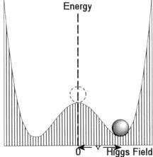
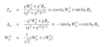
This form of field exhibits a drastic effect called "spontaneous symmetry breaking". When the origin of the field is shifted to v by the transformation ' = - v, the fields W^a and B recombine and reemerge as the physical photon field A, a neutral massive vector particle Z, and a charged doubled of massive vector particles W^+/-:

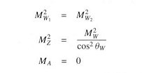
The masses of the gauge bosons are obtained from the mass sector:

Physically, the effect can be interpreted as an object moving from the "false vacuum" (where = 0) to the more stable "true vacuum" (where = v). Gravitationally, it is similar to the more familiar case of moving from the hilltop to the valley. In the case of Higgs field, the transformation is accompanied with a "phase change", which endows mass to some of the particles.

Experimentally, the predictions of the Weinber-Salam model have been tested to about one part in 10³ or 10⁴. It has been one of the outstanding successes of the field theory, gradually rivaling the predictive power of QED.

The above formulism can be carried over to the electro-weak interactions between quarks with the massless neutrino replaced by the up quark u (which has mass), and the electron replaced by the down quark d. In order to get the correct quantum numbers, such as the charge, the covariant derivatives are different from the lepton as shown below:

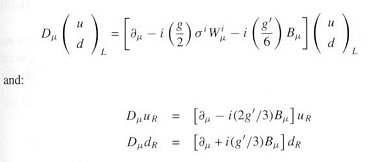
where the coupling constants g and g' are also different from the case of leptons.

The theory for the strong interaction is called quantum chromodynamics (QCD), which has the Lagrangian density:

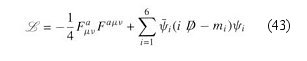
Since the gauge bosons (the gluons) are massless, the Lagrangian density appears to be in a much simpler form than the electro-weak interactions in Eq.(40).

Meaning of the symbols in the QCD Lagrangina density :

F^a is similar to the SU(2) gauge field in Eq.(42a). This is essentially the Yang-Mills field developed back in 1953 by generalizing the gauge invariance used in QED. It represents the eight massless gluons carrying the SU(3) "colour" force with the index "a" running from 1 to 8.
The index "i" is taken over the flavors, which labels the up, down, strange, charm, top, and bottom quarks. The flavor index is not gauged; it represents a global symmetry. However, the quarks also carry the local colour SU(3) indices red, green, and blue (which is suppressed here). In other words, quarks come in six flavors and three colours, but only the colour index participates in the local gauge symmetry. It is the colour force, which binds the quarks together.
= .
m_i denotes the mass for the various quarks.

The Lagrangian for the Standard Model then consists of three parts:
where WS stands for the Weinberg-Salam model, and lept. and qurk. stand for the leptons and quarks that are inserted into the WS model with the correct SU(2)XU(1) assignments. It is assumed that both the leptons and quarks couple to the same Higgs field in the usual way. From this form of the Standard Model, several important conclusions can be drawn. First, the gluons from QCD only interact with the quarks, not the leptons. Thus, symmetries like parity are conserved for the strong interactions. Second, the chiral symmetry, which is respected by the QCD action in the limit of vanishing quark masses, is violated by the weak interactions. Third, quarks interact with the leptons via the exchange of W and Z vector mesons.

Alıntı: http://universe-review.ca/R15-12-QFT.htm

Hiçbir yazı/ resim izinsiz olarak kullanılamaz!! Telif hakları uyarınca bu bir suçtur..! Tüm hakları Çetin BAL' a aittir. Kaynak gösterilmek şartıyla siteden alıntı yapılabilir.

Ana Sayfa /İndex /Roket bilimi / E-Mail /CetinBAL /Quantum Teleportation-2

Time Travel Technology /Ziyaretçi Defteri / UFO Technology

Kuantum Teleportation / Kuantum Fiziği / Duyuru

New World Order(Macro Philosophy)/Astronomy