Time Travel Research Center © 2005 Cetin BAL - GSM:+90 05366063183 - Turkey/Denizli
Classical Mechanics, Relativity, and Time
Contents
Classical Mechanics
Special Relativity
General Relativity
Time
Classical Mechanics
Classical mechanics describes the way objects move and interact in
accordance with Newton's laws of motion. The basic assumptions involve a
frame of reference (x,y,z) with respect to which the objects move, there is
an independent time variable t to record the sequence of the movement, the
gravitational or electromagnetic interaction between objects is
instantaneous, and objects with geometric extent are often idealized as a
point (with the justification that the size is much smaller than the
distance involved). The basic equation is:
F = m a ---------- (1)
This formula is known as the equation of motion and looks deceptively simple.
However, the force F and acceleration a are vectors, which
have to be resolved into the x, y, z components. The acceleration a
is the derivative of the velocity v, which is also a vector and the
derivative of the positional vector r, i.e., v = dr/dt.
The mass m is a proportional constant according to the Newton's second law.
If the positional vector r is decomposed into r = x i +
y j + z k, where i, j, and k are unit
vectors along the x, y, z axes respectively, then Eq.(1) can be written in
its component form:
Fx = d2x/dt2, Fy = d2y/dt2,
and Fz = d2z/dt2 ---------- (2)
which are essentially three separate differential equations. The force F
can be a sum of many forces acting together; if the resultant is zero then
the object is said to be in equilibrium and would not experience
acceleration. This is the Newton's first law. The Newton's third law is : in
his own words, "To every action there is always opposed an equal reaction;
or, the mutual actions of two bodies upon each other always equal, and
directed to contrary parts."
The Newton's law of universal gravitation is in the form:
F = (Gm1m2 / r2) (r/r)
---------- (3)
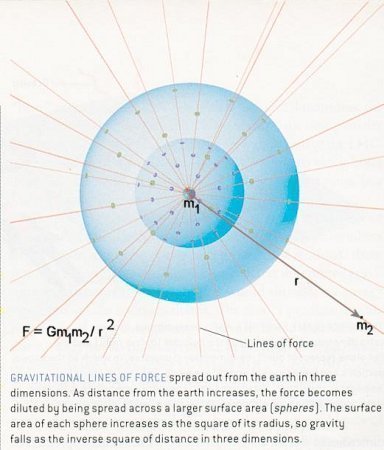
where G is the gravitational constant, m1 and m2 are
the masses of the two objects interacting via gravitation, r is the distance
between these two objects, and (r/r) is an unit vector along the
direction of r as shown in Figure 01 below:
m1 r m2
o----------------------------o
r/r =>
Figure 01 Gravitational Interaction
If one of the objects is much heavier than the other, e.g., m1 >>
m2 like the Sun / Earth system, then m1 can be placed
in the origin of the coordinate system and Eq.(1) can be solved as a one-body
problem. In case the two masses are similar, the problem can be reduced to a
one-body problem with a fictitious object moving around the center of mass,
and Eq.(1) is still applicable. The equation of motion becomes rapidly un-manageable
for system of three bodies and beyond. Eq.(1) would include accelerations
for all the objects and the force on one object would involve the
interaction with all the others. This is the situation often encountered in
celestial mechanics with spacecraft flying among planets. The solution is
usually obtained by some kind of approximation and by numerical computation
using large computers.
Now consider two frames of reference S and S'. The S' system is coincided
with S at t = 0 and moving with a constant velocity V along the x axis as
shown in the diagram below:
S|_____x1_____x2_____ x S'|________________
x' ===> V
Figure 02 Equivalent Inertial Frames of Reference
The transformation between these two coordinate systems (known as inertial
frames of reference) can be expressed by the Galilean transformation:
x' = x - Vt, y' = y, z' = z, and t' = t ---------- (4)
It is obvious that the length L = x2 - x1 = L' = x'2
- x'1, i.e., it remains unchanged in the two coordinate systems.
In general, the invariant form of the infinitesimal length of an object can
be expressed as:
dx2 + dy2 + dz2 = dx'2 + dy'2
+ dz'2 ---------- (5)
It can be shown that the gravitational force in Eq.(3) together with the
equation of motion in Eq.(1) are also invariant under the Galilean
transformation. However, according to the formula in Eq.(4) the velocity of
light c would be different with c' = c - V.
Special Relativity
It had been demonstrated by Michelson and Morley in 1887 and others that the speed of light in free space is the same everywhere, regardless of any motion of source or observer. The Maxwell's equations in electromagnetism also indicates that the speed of light is an absolute constant regardless of the relative motion of the person measuring that speed. But as just mentioned above, the velocity of light is different in different inertial frame according to the Galilean transformation. The theory of special relativity was postulated to reconcile the inconsistency from these kinds of observations. Mathematically, the statement about the constant velocity of light in different inertial frames can be expressed as:
x2 + y2 + z2 = c2 t2
---------- (6)
x'2 + y'2 + z'2 = c2 t'2
---------- (7)
if a spherical light wave is generated at the origin of the S and S'
inertial frames when they are coincided at t = 0. This situation is possible
only when t is not equal to t'. It can be shown that the Lorentz
transformation below would satisfy the requirement in Eq.(6) and (7):
x' = (x - Vt) / (1 - V2/c2)1/2, y' =
y, z' = z, and t' = (t - Vx/c2) / (1 - V2/c2)1/2
---------- (8a)
The inverse transformation is:
x = (x' + Vt) / (1 - V2/c2)1/2, y =
y', z = z', and t = (t' + Vx'/c2) / (1 - V2/c2)1/2
---------- (8b)
Eq.(8a) reduces to the Galilean transformation in Eq.(4) when V/c << 1. In
this way, x, y, z, and ct form a four-dimensional space known as the
Minkowski space-time. It revolutionizes high-energy physics when velocity of
the particles is close to the velocity of light (relative to the observer's
inertial frame). All the basic formulae such as the field equations and the
Lagrangians have to be invariant under the Lorentz transformation, and the
definition for many physical entities changes form at high speed as listed
in the followings:
- The independent time variable t is now treated on the same footing as the other spatial dimensions.
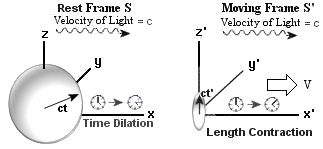
- The length L' = x'2 - x'1 in the moving inertial
frame is now different with respect to a stationary observer in the S
system
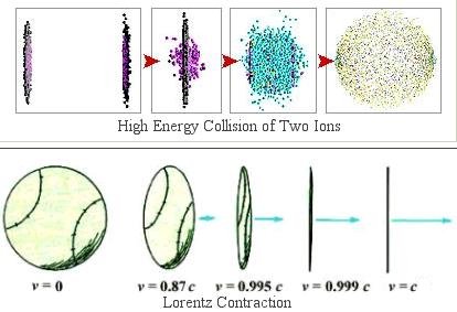
at t = to. According to the 1st formula in Eq.(8a), the relation is given by: L = x2 - x1 = L' (1 - V2/c2)1/2, which is known as the Lorentz contraction. The length of a moving rod is shorter according to a stationary observer. The phenomena is demonstrated in high energy collision, when the round shape of atom becomes a pancake with the flatten face perpendicular to the direction of motion (see Figure 03). Figure 03 Lorentz Contraction
Figure 04 Time Dilation
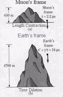
- The time interval T' = t'2 - t'1 of a clock
sitting in the S' system at x' = x'o appears to take longer to
tick with respect to a stationary observer in the S system. According to
the 4th formula in Eq.(8b), the relation is given by T = t2
- t1 =
T' / (1 - V2/c2)1/2. The effect is known as time dilation and T' is referred to as the proper time - the time experienced in the clock's rest frame. The phenomena is demonstrated in the decay of unstable particle moving at near the speed of light. The lifetime of such particle appears to be much longer than the one measured in a stationary lab. The diagrams in Figure 04 (where = (1 - V2/c2)-1/2),
show the muon decay as experienced in its own frame and from the view
point of a stationary observer on Earth.
= (1 - V2/c2)-1/2),
show the muon decay as experienced in its own frame and from the view
point of a stationary observer on Earth.
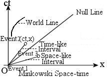
- Events (a point in the four dimensional space-time as shown in Figure 05) that take place simultaneously to an observer in S, e.g., t = to at x = x1 and x = x2, are separated by a time interval t'2 - t'1 = (V(x1 - x2)/c2) / (1 - V2/c2)1/2 in S' according to the 4th formula in Eq.(8a) (see Figure 06).
- For an infinitesimal interval of space-time, Eq.(6) can be written in the form:
dx2 + dy2 + dz2 - c2 dt2 = 0 ---------- (9)Figure 05 Reference Frame
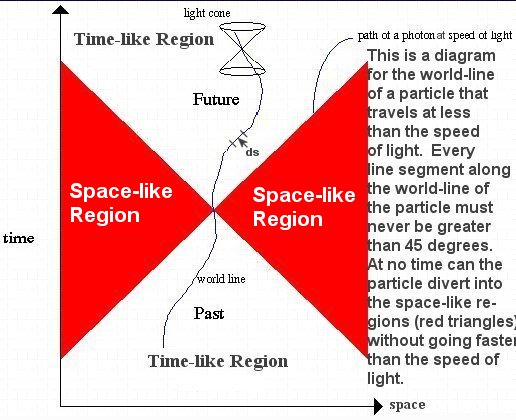
This is called the null line applicable to object moving at the speed of light. It can be shown that the space-time interval
ds2 = dx2 + dy2 + dz2 - c2 dt2 ---------- (10)
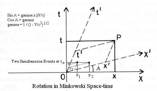
Figure 06 Rotation in Minkows- ki space-time
is invariant under the Lorentz transformation. ds is called proper interval because it is related to the interval for an object at rest with dx = dy = dz = 0. The interval is called time-like if ds2 < 0. In this case, Event 2 can be related causally in some way to Event 1 provided that a signal (traveling slower than the speed of light) is available. If ds2 > 0, then it is called space-like, which implies Event 3 is entirely unrelated to Event 1. Alternatively it can be interpreted that two events joined by a space-like interval can never influence each other, since that would imply a flow of information at speeds faster than the speed of light (see Figure 05).
- It is obvious from Eq.(10) that it is actually ict, which becomes the 4th dimension in special relativity. This is the reason for the un-usual appearance of the space-time axes when subject to a rotation in the Minkowski space-time (Figure 06).
- In Galilean transformation the velocity in the S' system is v' = v -V, which is now replaced by v' = (v - V) / (1 - vV/c2) in special relativity.
- The mass for a particle moving at velocity V is given by m = mo / (1 - V2/c2)1/2, where mo is the rest mass (relative to the observer's inertial frame).
- Mass and energy are equivalent. They can be converted to each other. The total energy E of a particle is given by the formula E = m c2 = mo c2 + T. The first term is the rest mass energy, and the second term is the kinetic energy.
- In term of the momentum p, E = (mo2 c4 + p2 c2)1/2.
General Relativity
 |
 |
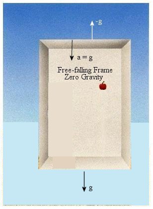
The inertial frames of reference in both classical mechanics and special relativity move with a constant velocity related to each others. Such arrangement seems to become impossible in the presence of gravity, which produces acceleration (change of velocity). However, there is a class of frames of reference that can be obtained locally by letting it freely falling. This kind of frames would generate an opposite force, which exactly nullifies the acting force. The local region (such as in an |
Figure 07 Free-falling Frame |
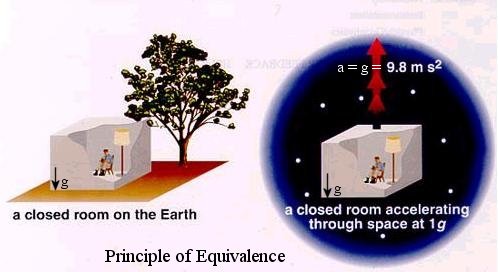
Figure 08 Equivalence Principle
|
elevator) would experience zero gravity as shown in Figure 07. Figure 08 shows the similar kind of situation in producing gravity with acceleration. The inter-changeable nature of gravity and acceleration is known as the principle of equivalence. |
The space-time interval in Eq.(10) is valid as long as the observer is
confined to the free-fall frame of reference (inside the elevator). Since
the gravitational field is not uniform in general, the frame of reference
will follow a curved world line (a line traced out by 4 dimensional events,
it is a straight line for constant velocity motion) as shown in Figure 05,
which depicts the path of a particle accelerating from rest up to the
velocity of light. In order to describe this kind of motion globally, Eq.(10)
is now replaced by a more general form taking into account the unevenness of
the field:
ds2 = gik dxi dxk ----------
(11)
where the notations have been simplified such that x = x1, y = x2,
z = x3, ct = x4; the indices i, k run from 1 to 4 and
denote a summation whenever it is paired (in the subscript and the
superscript). The gik is known as space-time metric, which is a
second rank tensor and a function of the space-time. In an inertial frame (flat
space-time), g11 = g22 = g33 = 1, g44
= -1, gik = 0 for i ¬= k. In general the space-time metric gik
is determined by the nonlinear differential equations as postulated by
Einstein:
Rik = (8![]() G/c4)
(Tik - gikT) ---------- (12)
G/c4)
(Tik - gikT) ---------- (12)
where Rik is a second rank tensor related to the curvature of
space; it involves the first and second derivatives of gik; Tik
(and T = Tii) is the energy-momentum tensor of matter-energy.
Thus, gravity is geometrized and the geometry of the space-time is
ultimately determined by matter-energy.
The equations of gravitational field can be solved exactly for the case of a
centrally symmetric field in vacuum with mass m at the center. In terms of
spherical coordinates and ct, it has the form:
ds2 = dr2 / (1 - 2Gm/c2r) + r2
(sin2![]() d
d![]() 2
+ d
2
+ d![]() 2) - (1 - 2Gm/c2r)
c2dt2 ---------- (13)
2) - (1 - 2Gm/c2r)
c2dt2 ---------- (13)
This is known as the Schwarzschild solution. It is a useful example for
illustrating the many properties in general relativity:
- At large distance from the center, where r approaches infinity, the space-time metric reduces to the flat space-time.
- At sufficiently large distances, where r >> 2Gm/c2, the
solution assumed the characteristics of the classical inverse-square law
of gravitation in the following form:
ds2 = (1 + 2Gm/c2r) dr2 + r2 (sin2 d
d 2
+ d2) - (1 - 2Gm/c2r)
c2dt2 ---------- (14)
2
+ d2) - (1 - 2Gm/c2r)
c2dt2 ---------- (14) - At the distance where r = rs = 2Gm/c2, the escape velocity ve = (2Gm/r)1/2 = c. It implies that even light cannot escape the grip of gravity at this point. This is Schwarzschild radius separating the black hole from the rest of the world.
- A black hole can form only when the Schwarzschild radius rs is outside the central object. For the Earth, and the Sun, rs is well inside the physical boundary (rs for the Earth is about 1 cm anf for the Sun is about 3 km). Even the neutron star (with similar mass to the Sun) has a physical radius of about 10 km. Only collapsing stars or galactic center have the necessary condition to form a black hole.
- Gravitational redshift is generated as the photons loss energy in
overcoming the pull of the gravitational field. For the case of spherical
mass at the center, the shifted wavelength is computed by the formula:
 =
o (1 - rs/r)-1/2
---------- (15)
=
o (1 - rs/r)-1/2
---------- (15)
At the Schwarzschild radius rs, the redshift becomes infinity. This is the effect that makes light invisible at rs. - The gravitational field also induces time dilation as experienced by a
far away stationary observer. It is in a similar form as Eq.(15):
T = To (1 - rs/r)-1/2 ---------- (16)
where To is the time interval recorded by an observer plunging toward the black hole and T is the corresponding time perceived by a stationary observer. Thus, for the stationary observer it takes an infinite long interval for the other observer approaching the Schwarzschild radius rs. However, the adventurer is not aware this curious effect on the time interval. His journey may be interrupted only by the tidal force, which is much more ferocious for black hole with smaller size (the tidal force at rs is proportional to 1 / m2). - Inside rs, all matter must fall towards the center, even
light, which keeps coming from outside (but cannot get out from inside).
After a finite time the inward falling object will end up at r = 0, where
the density of matter is infinite. The metric g44 changes sign
inside the black hole, i.e., time has become just another dimension of
space. It is suggested such change has the effect of smoothly rounded off
the singularity at r = 0.
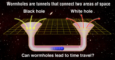
Figure 09 Schwarzschild Solutions
- White holes are similar to black holes except white holes are ejecting matter while black holes are absorbing matter. The existence of white holes is implied by a negative square root solution to the Schwarzchild metric. If we define the proper time d
 to be the time associated with the moving frame, in which the spatial
variation vanishes (co-moving objects are stationary in that frame),
then
to be the time associated with the moving frame, in which the spatial
variation vanishes (co-moving objects are stationary in that frame),
then c2 d
2
= -ds2 = -g44 c2 dt2
where g44 is negative according to the convention. Thus,
d = ± (-g44)1/2
dt
where the positive sign corresponds to the black hole solution while the solution with negative sign is interpreted as the with hole with time running backward (see Figure 09). - White holes are similar to black holes except white holes are ejecting matter while black holes are absorbing matter. The existence of white holes is implied by a negative square root solution to the Schwarzchild metric. If we define the proper time d
- Inside the Schwarzschild radius, g11 and g44 change sign as shown in Eq.(14). It is possible to create another geometry, which prevents the formation of a singularity and forms a tunnel known as the Einstein-Rosen Bridge or wormhole. Even though mathematically this bridge is allowed to exist, physically it is doomed to collapse; the gravitational forces are completely overwhelming. However if there is a large amount of negative energy to sustain the structure, then a wormhole may remain open. This would allow for travel within the wormhole between two distant points, or to even allow for the possibility of "time" travel (see Figure 09).
Blackholes
 |
 |
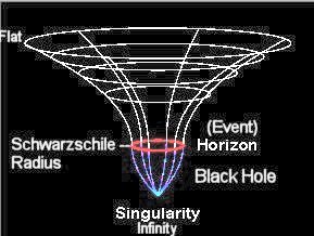
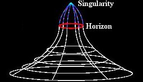
The concept of black hole has its origin in a solution of Einstein's General Relativity for a spherical object with mass M and radius R. If the mass collapses to a radius less than R = 2xGxM/c2, where G is the gravitational constant and c is the speed of light, then nothing (including light) can escape from inside this radius. It is called the event horizon or the Schwarzschild radius (named after the astrophysicist who solved the equation). Figure 05-06a shows a schematic diagram of the Schwarzschild geometry. |
Figure 05-06a Black Hole |
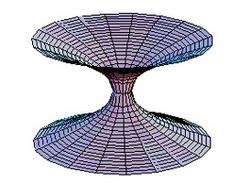
Figure 05-06b Worm Holes |
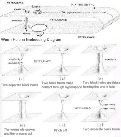
It is known as the embedding diagram. The two dimensional circles are
slices of three dimensional spheres (of the same radius) - the hyperspace.
The verticle axis denotes the "stretch" of space in the radial direction.
The slope of the curve can be considered as representing the curvature of
the space. It is flat (or zero) at the outer edge and becomes infinity at
the Schwarzschild radius. This pictorial representation is very similar to a
rubber sheet stretched by
a rock. The shape of the region inside the horizon is somewhat arbitrary.
It is only known that everything plunges inevitably to the central
singularity once passing over the horizon. In a more realistic drawing the
event horizon would be placed far below the diagram at infinity. The
complete Schwarzschild geometry consists of a black hole, a white hole, and two singularities connected at their horizons by a
worm hole
as shown in Figure 05-06b. A white hole is a black hole running backwards in
time. Just as black holes swallow things irretrievably, so do white holes
spit them out. White holes cannot exist, since they violate the second law
of thermodynamics by allowing some time reversal events such as reassembling
a broken glass back to its original whole. The white hole geometry outside
the horizon represents another Universe. The worm hole joining the two
separate singularities is known as the Einstein-Rosen bridge, but even if it
can somehow be generated, it would be unstable and pinch off immediately.
Therefore, only the black hole geometry is applicable to the physical world.
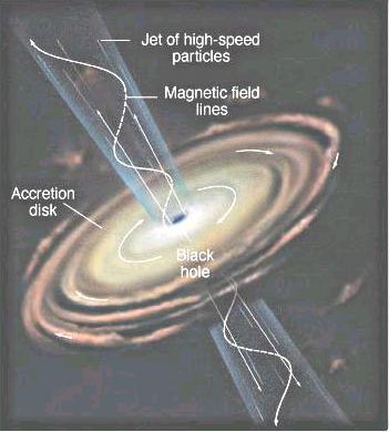 |
It is believed that every quasar, active galactic nucleus, and even normal galactic nucleus contains a black hole with a mass of between ten million to several billion solar masses at its core. The difference in appearance is related to the intensity of the activity. Since galaxies rotate, matter falling toward the central black hole will form a rapidly spinning disk of gas - an accretion disk - rather than falling directly into the hole. Kinetic energy released by in-falling matter, and frictional effects within the accretion disk, raise the temperature of the nner parts of the disk to enormous values and provide plenty of energy to power AGN's on all scales from Seyferts to quasars. By a process that is still not fully understood, the central engine accelerates streams of charged particles to very high speeds. The inner rim of the accretion disk, together with surrounding gas and magnetic fields, forms a nozzle that confines the outward flow of energetic particles into narrow streams that shoot out perpendicularly to the plane of the disk. The lower half of Figure 05-07a shows a model of the black hole. |
Figure 05-07a AGN Model |
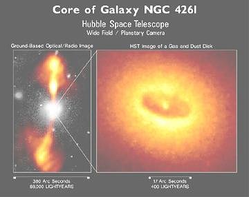
Figure 05-07b is a HST (Hubble Space Telescope) image of NGC4261, which is a radio galaxy. The image strongly suggests that it is a black hole fitting the description of the theoretical model. Infrared observation of NGC1068 in 2004 was able to resolve the inner region down to a few parsec. Figure 05-07c penetrates the dusty central region and shows the structures on arcsec scales. The picture on the right is a model for the nucleus of NGC1068. It contains a central hot component (dust temperature > 800K, yellow) marginally resolved along the source axis (dashed line). Its finite width and the dashed circle indicate the currently undetermined extent. The much larger warm component (T=320K, red) is well resolved. The arrows
 |
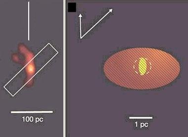 |
indicate the projected orientation of the two interferometer baselines and the angular resolution L/2B, where L is the wavelength and B is the projected baseline. The image shows that the active galactic nuclei are arranged like a thick doughnut. This model requires a continuous injection of kinetic energy to maintain such cloud system. The mechanism is currently unknown; thus a better understanding of the physics of these spectacular objects is needed. |
Figure 05-07b NGC4261 |
Figure 05-07c NGC1068 |
The quasar 3C273 is a 2-billion-solar-mass black hole encircled by a doughnut of gas (accretion disk) and with two gigantic jets shooting out along the spinning axis. The Schwrzschild radius for this object is about 6x10⁹ km. Such supermassive black hole can be created while matter is still at quite low density (~ 10-3 gm/cm3). Since the tidal force at the event horizon of a black hole is inversely proportional to the square of its mass, its effect on a space visitor would be un-noticeable, although he would soon be in dire trouble as he plunges irrevocably toward the central singularity. However for a stationary observer, it takes an infinitely long time for the asronaut to approach the event horizon (due to gravitational time dilation) and the view of the asronaut would gradually disappear (due to gravitational red shift of light). The effect on the astronaut visiting a stellar black hole (mini-quasar) would be more violent due to the drastic increase of the tidal force.
Another example that offers exact solution is the homogeneous and isotropic space filled with pressure-less dust. It is applicable to the case of the cosmic expansion, if each dust point presents a galaxy. Universes of this type are variously known as Friedman universes, Friedman-Robertson-Walker universes, ... etc. The effect of radiation energy, which is important in the very early universe and the cosmological constant, which may be responsible for the cosmic repulsion are neglected in the following consideration.
- The space-time interval is associated with the Robertson-Walker metric.
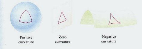
It has three forms depending on the curvature of the 3
dimensional space:
ds2 = R(t)2 (dw2 + s2 (sin2
d2 + d2)
- c2dt2 ---------- (17)
where s = sin(k1/2 w) / k1/2, and R(t) is called the scale factor.
For flat space with zero curvature, k = 0, and s = w.
For closed space with positive curvature, k = +1, s = sin(w), where w ranges from 0 to 2 .
.
For open space with negative curvature, k = -1, s = sinh(w), where w ranges from 0 to infinity.
- In term of the Robertson-Walker metric and with the energy-momentum
tensor T00 =
 , the
gravitational field equation becomes:
, the
gravitational field equation becomes:
(dR/dt)2 + kc2 = 8 GR2
/ 3 ---------- (18a)
GR2
/ 3 ---------- (18a)
It can be re-arranged into the form:
k2 c2 = H2 R2 ( - 1) ---------- (18b)
if we define the Hubble parameter H(t) = (dR/dt) / R, the critical densityc = (3 H2)
/ (8G), and
=
/
c.
By inspecting Eq.(18b), it is obvious that
for flat space, =
c,
= 1, and k = 0;
for closed space, >
c,
> 1, and k = +1;
for open space, <
c,
< 1, and k = -1.
- If we choose = M / (4R3/3),
where M may be interpreted as the total mass of the universe, Eq.(18a)
becomes:
(dR/dt)2 + kc2 = 2GM / R ---------- (18c)
The solution for this equation is:
for k = 0, R = (9GM/2)1/3 t2/3 ---------- (19a)
for k = +1, R = Ro (1 - cos(µ)), ct = Ro (µ - sin(µ)) ---------- (19b)
where Ro = GM / c2, and µ is defined by c dt = R(t) dµ.
for k = -1, R = Ro (cosh(µ) - 1), ct = Ro (sinh(µ) - µ) ---------- (19c)
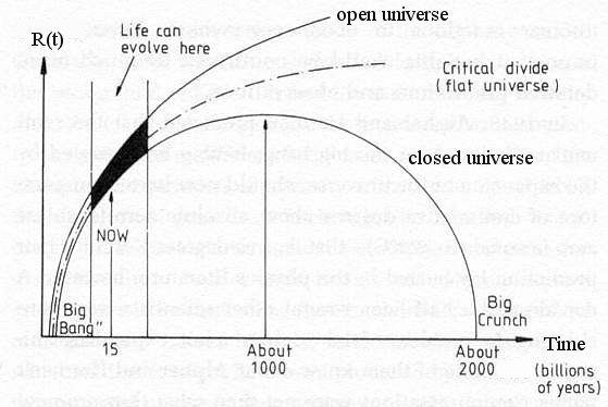
- Figure 10 shows the three types of universe - open, flat, and closed. Universes that are too far above the critical divide expand too fast for matter to condense into stars and galaxies; such universes therefore remain devoid of life. Those that fall too far below the critical divide collapse before stars have a chance to form. The shaded area indicates the range of cosmological expansions and epochs in which observers could evolve. Recent type Ia supernova data seems to indicate an open universe with acceleration.
Figure 10 Types of Universe
The equation of motion in relativity is the geodesic (shortest path) for
a particle moving in space-time:
d2xi/ds2 +
![]() ikl (dxk/ds)
(dxl/ds) = 0 ---------- (20)
ikl (dxk/ds)
(dxl/ds) = 0 ---------- (20)
where ![]() ikl
is in terms of the metric tensor and its first derivative. It is known as
the Christoffel symbols. For
ikl
is in terms of the metric tensor and its first derivative. It is known as
the Christoffel symbols. For
![]() ikl
= 0 Eq.(20) reduces to the usual equation of motion of a free particle.
ikl
= 0 Eq.(20) reduces to the usual equation of motion of a free particle.
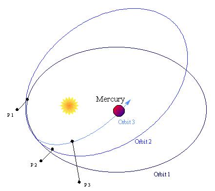 |
Using the gravitational field equation and the equation
of motion, Einstein presented a calculation on the effect of GR on the
advance of the perihelion of Mercury: where M is the mass of the Sun, a is the length of the semi-major axis, and e is the eccentricity of the ellipse. In Figure 11, the amount of the advance is greatly exaggerated. The actual advance due to the effect of GR is only 0.43 seconds of arc per year. The most recent and most accurate results seem to be converging towards a value that makes the GR predictions agree well with observation. |
Figure 11 Perihelion Advance |
Time
A brief history of time and beyond:
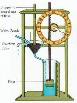 |
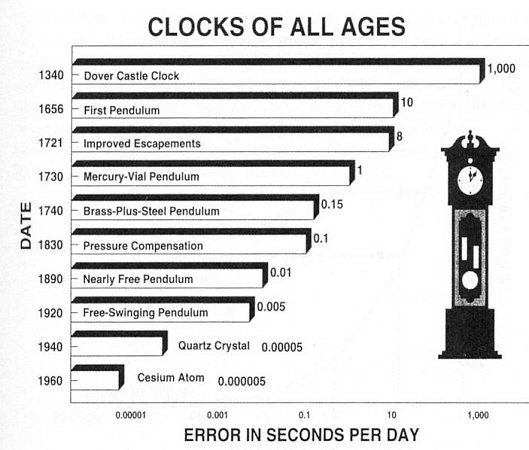
For 10 billion years, the universe has been in existence without bothering with the definition of time. It started about 3.5 billion years ago when unicellular organisms took up residence on Earth. They had to adjust their activities according to the daily and yearly cycles. Since then all living beings including human come equipped with biological clocks within to adopt to these rhythms. For thousands of years, protohumans probably had only dim notions of time: past, present, and future. Beginning around 2500 BCE, systemic definitions of time were developed in the form of calendars. The Egyptian pioneers first divided a day into 24 units. Other calendars were linked to religion and the need to predict days of ritual significance, such as the summer solstice. All calendars had to resolve the incommensurate cycles of days, lunations and solar years, usually by intercalating extra days or months at regular intervals. The Julian calendar was established at 46 BCE. The first mean of measuring daily time was probably the Egyptian shadow stick, dating from about 1450 BCE. It was soon followed by the water clock or clepsydra (Figure 12) and the sandglass or hourglass, in which time is measured by the change in level of flowing water or sand. The |
Figure 12 Clepsydra |
earliest mechanical clocks containing movable parts were
built about 700 years ago. It had no minute hand. |
When Newton published the three natural laws in 1686, time is no longer
confined to record the daily and yearly rhythms. It had become a
mathematical entity - a parameter to keep track of motions in a fixed,
infinite, unmoving space. Einstein changed all this with his relativity
theories, and once wrote, "Newton, forgive me." In the new theories, time is
treated almost on the same footing as the other spatial dimensions with some
minor differences. Recently, theory in quantum gravity considers time
and space to be discrete at the Planck scale with a minimum size of about 10
-43 sec and 10-33 cm respectively. At this scale, they
are useless as framework for the motion of other objects. It is suggested
that time and space are the active participants in the dynamics of this
world.
In place of space and time as parameters to describe the evolutions of
systems, the modern approach is to introduce the artificial time (T)
and artificial spatial coordinates (X1, ..., Xn),
which have nothing whatsoever to do with real time and real space. Since
nobody has ever seen or detected the artificial space-time, they have to be
un-observable in the mathematical formulation. Such theories are said to be
reparametrization invariant because they are not affected by the change to
another set of artificial space-time parameters. This is sometimes referred
to as the unobservability principle. It then more or less leads to the
string theory, which is reparametrization and
conformally (change of scale)
invariant.
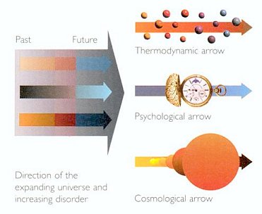
- The arrow of time - The laws of physics do not care about the direction of time, i.e., the mathematical formulations are invariant if the direction of time is reversed. Yet there is a big difference between the forward and backward directions of real time in ordinary life. We have no difficulty to tell the sequence of events in Figure 13 (from 1 to 9), because it is highly improbable for the crumbling dust to return to the structured building in the
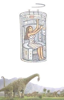
- It is strongly suspected that general relativity also preserves causality and forbids agents from changing the past, although this has not been rigorously demonstrated. The idea of using time machine to visit the past is still a hot topic.
- The psychological time - The psychological perception of time is affected by such things as medications, time of day, level of happiness, external stimuli, and even the temperature. Einstein once remarked, "When you spend two hours with a nice girl, you think it's only a minute. But when you sit on a hot stove for a minute, you think it's two hours." Thus, the time line experienced by the conscious brain is often quite different from the "objective" time line of events occurring in the real world.
- Cosmological arrow of time - Since volume expansion tend to increase the entropy of a system, the cosmic expansion seems to be a good indicator for the direction of time (Figure 12b). But what would happen if and when the universe stops expanding and begins to contract? According to Hawking, he used to believe that disorder would decrease when the universe recollapse. Now he realizes that the no boundary condition implies that disorder would in fact continue to increase during the contraction. He attributes the association between the thermodynamic and cosmolgical arrows to the no boundary condition instead of volume expansion.
Instead of trying to define time or provide an answer to the
philosophical question of "What is time?", some of the characteristics of
time are listed in the followings:
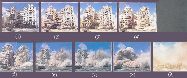
Figure 13 Arrow of Time
|
|
| reversed direction. This is usually explained by the second law of thermodynamics, which states that in the macroscopic world there is a tendency for a closed system moving toward greater disorder. |
Figure 12b Arrows of Time

|
  |
 |
|
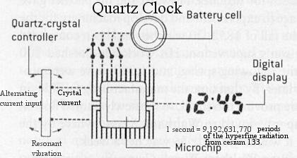
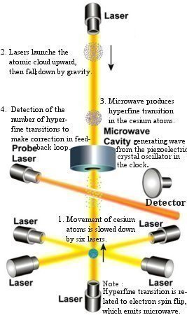
Figure 14 Clocks |
Figure 15 Atomic Clock |
Atomic clocks use the frequency of vibration of atoms to regulate a quartz crystal clock (see Figure 15). One second is now defined as the duration of 9,192,631,770 periods of the radiation from the hyperfine transition of the cesium atom. |
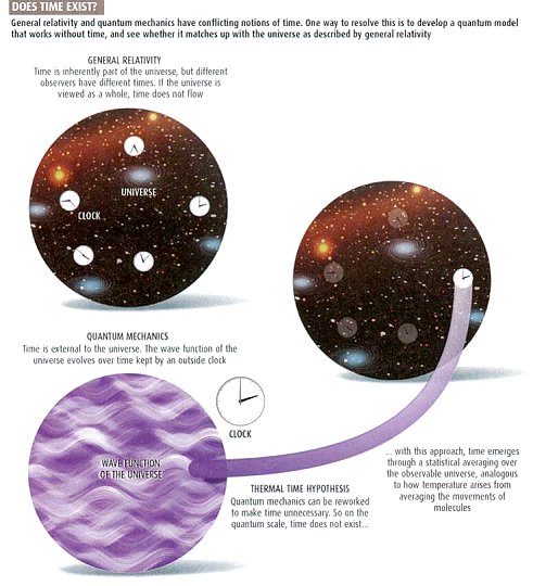
- End of time - Recently, there is suggestion that time is just an illusion. Time as such does not exist. There is no invisible river of time. But there are things that can be called "instants of time", or "Nows". As we live, we seem to move through a succession of Nows. The idea is that when we think we are seeing actual motion, the brain is interpreting all the simultaneously encoded images and playing them as a movie - frame by frame. Mathematically, it is similar to plot points in the phase space, where the element of time is left out. It has to rely on either color codes (for example, blue for earlier and red for later moment) or animation to display the evolution of the system. In this way, time is just replaced by something else.
- Imaginary time - The imaginary time T is defined by: t
 it'. This
simple substitution is rather controversial in the community of
theoretical physicists. Some argue that it is merely a mathematical trick,
or a convenient tool devoid of any physical significance. Others suggest
that imaginary time is the true physical quantity. Whatever its merit,
imaginary time does provide an alternate computational technique and
conceptional viewpoint as shown in the following examples (Note that
imaginary and real are just mathematical terminologies in this context. It
has nothing to do with the usual connotation of mental perspective.).
it'. This
simple substitution is rather controversial in the community of
theoretical physicists. Some argue that it is merely a mathematical trick,
or a convenient tool devoid of any physical significance. Others suggest
that imaginary time is the true physical quantity. Whatever its merit,
imaginary time does provide an alternate computational technique and
conceptional viewpoint as shown in the following examples (Note that
imaginary and real are just mathematical terminologies in this context. It
has nothing to do with the usual connotation of mental perspective.).
Quantization of particles and fields is most elegantly prescribed by the method of path integral. The mathematical formula in term of the real time t for the probability amplitude to go from q(t1) to q(t2) is proportional to:
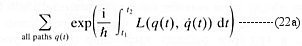
where the sum is over all paths and L is the Lagrangian (a function of the position and velocity). The oscillating factors in this formula are very difficult to manipulate. However by substituting the real time with the imaginary time, Eq.(22a) is changed into:
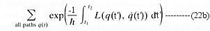
which become the more manageable exponentially decreasing functions. At the end of the computation, the imaginary time can be switched back to the real time.
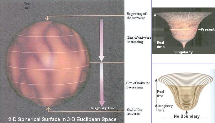
Figure 15a The "No Boundary" Proposal
Meanwhile, if the imaginary time is substituted intoEq.(10), it changes into a form familiar to Euclidean geometry:
ds2 = dx2 + dy2 + dz2 + c2 dt'2 ---------- (23)
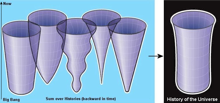
While the real time in Eq.(10) restricts the time direction within the light cone, for the imaginary time there is no difference between the time direction and directions in space. Thus according to Hawking, it is possible for such space-time to be finite in extent and have nosingularities that formed a boundary or edge. As shown in Figure 15a, space-time would be like the surface of the earth, only with two more dimensions. Such Euclidean sphere has zero points at the North and South Poles, but these points would not be any more singular than these Poles on earth. The corresponding universe in real time would have a minimum size, which corresponds to the maximum radius of the history in imaginary time. At later real times, the universe would expand at an increasing inflationary rate to a very large size (see lower right diagram in Figure 15a or Figure 10n). By combining the two examples as illustrated above, a path integral similar to Eq.(22b) can be used to calculate the probability amplitude for the no boundary universes. The sum over histories is actually
performed backward in time from the current state of the universe such as three-dimensional and flat, then construct the set of all possible histories that would end up like ours (with variables such as inflation, big crunch, ...), and finally sum them up by assigning a weighting factor to each to produce the probability amplitude for the history of a certain universe (see Figure 15b). Although the answer matches observations (i.e., our universe is the most probable) and incur no singularity, many physicists argue that this is just giving up on the problem of explaining why our universe is the way it is - it is not, they say, science. Figure 15b Sum over Histories
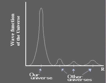
It can be shown that the probability amplitude for a particular history of the universe is related to the Wheeler-DeWitt Equation (which looks like the zero energy time-independent Schrodinger equation):
[ d2 / d R2 - U(R) ] = 0
---------- (23)
= 0
---------- (23)
where R is the scale factor, U is the potential (a function of R, the curvature, the cosomological constant, the densities of matter, and radiation), and is the wave
function of the universe, in which the particle position is replaced by the radius R for a multitude of universes. The result confirm that the expanding isotropic universe similar to our own is the most probable one (see Figure 15c). Figure 15c Wave Function of the Universe
- End of time (Figure 17) - Recently, there is suggestion that time is
just an illusion. Time as such does not exist. There is no invisible river
of time. But there are things that can be called "instants of time", or "Nows".
As we live, we seem to move through a succession of Nows. The idea is that
when we think we are seeing actual motion, the brain is interpreting all
the simultaneously encoded images and playing them as a movie - frame by
frame. Conceptually, it is similar to plot points in the phase space,
which is also known as configuration space where the element of time is
left out. Figure 18 depicts a very simple configuration space for an
universe of three particles A, B, and C. The lengths of each side (of the
triangle) form the three grid axes AB, BC, and CA. The seven triangles
represent several possible arrangements or NOWs of the model universe. The
black diamond indicates the position of each of these triangles or NOWs in
the configuration space. In general if there are n particles, the
configuration space will be constructed with n grid axes. We have no
access to the past and future. The past is only in our memories or some
sort of records. They are actually a present phenomena. The future is the
not yet realized events equally inacessible. We only experience a
continuous sequence of NOWs one after the other. Time was invented for the
convenience of human to keep track of
the changing NOWs. Note that the represent-ation in phase space is background independent. The spatial coordinates x, y, z are absent in the picture, and so is the time. Essentially, this is the foundation of the so-called relational theory in which all that matters is the relationships or links between the events. It plays a crucial role in the formulation of loop quantum gravity, in which space and time are discrete quantities and evolve dynamically like the atoms. Figure 18 Configuration Space
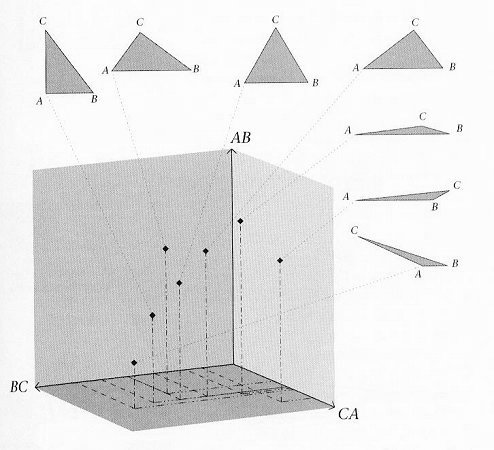
Figure 17 End of Time

- Another attempt to do away with time asserts that it is all an illusion. The thermal time hypothesis (Figure 19) suggests that a statistical effect gives rise to the "appearance" of time. Similar to temperature, which is the average of the momentum of each molecule, the same applies to the thermal time but including many more constituents such as space (which is expanding on the average). It predicts that the ratio of the observer's proper time to the thermal time is the surrounding temperature. A toy model has been constructed successfully from the CMBR data to explain the cosmic expansion as described by standard cosmology. It can also reproduce the temperature of a black hole associated with the Hawking radiation. The idea follows the rework of quantum mechanics without time. The evolution in time is replaced by the variation of correlations between things as mentioned above. Instead of "collapsing" the wave function of an electron, both the electron and the measuring device are described by a single wave function, and a single measurement of the
entire set-up causes the collapse. It is anticipated that combining quantum mechanics with general relativity would become less daunting when it is rewritten in time-free form. The loop quantum theory is an example adopting such idea. Figure 19 Thermal Time
 |
|
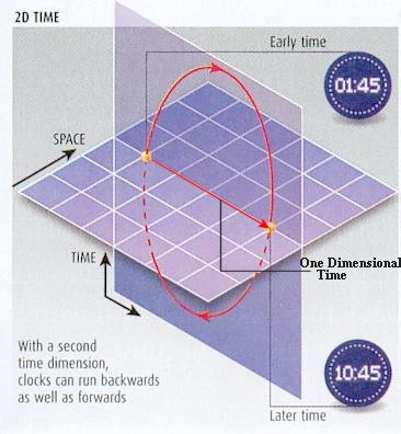
Figure 20 Two Dimensional Time |
For example, the problem associated with the
axion (a
not yet observed entity) can be resolved by the application of 2D-time
physics without such hypothetical particle. |
Figure 10r Warped 5-D
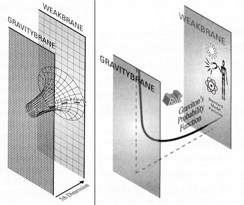
| An interesting application of warped 5th dimension has been developed by Lisa Randall. In this model, the 5th dimension is located in between two 3-D branes. It is found that the extra dimension is severely warped in the form of de Sitter space with positive curvature by the presence of bulk and brane energy even though the branes themselves are completely flat (see Figure 10r). The strength of gravity depends on the position of the 5th dimension. As shown in Figure 10r (in term of graviton's probability function), it can be very strong on the Gravitybrane but becomes feeble on the Weakbrane where all the forces and particles in the Standard Model are confined. Only the gravitons can move anywhere in the branes and in the bulk. This model explains why gravity is weak in our world although it can be |
| very strong in another brane. It also introduces a new way to solve the hierarchy problem of huge difference in mass between the Planck scale and the Electro-weak scale. If the Planck scale mass is set at the Gravitybrane, then the mass of particles on the Weakbrane would be reduced by a factor of 1016 to the Tev range as expected. |
Gravitational Wave
In the weak field limit where the space-time metric tensors gik
deviate only a small amount from flat space-time, the gravitational field
equation (12a) is reduced to the form:
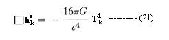
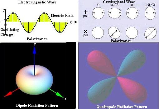
Figure 10s EW and GW
where the hki is small correction to gki,
Tki is the energy-momentum tensor, and
![]() is the d'Alembertian
operator in four-
is the d'Alembertian
operator in four-
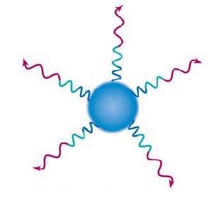
| dimensional space-time. This equation looks similar to the electromagnetic wave equation except that it is now a second rank tensor field (with 10 components) instead of the more familiar vector field. It is responsible for many different characteristics in these two kinds of field. Figure 10s shows the differences in polarization and radiation pattern. There are two polarization states in gravitational wave. They alternatively squeeze and stretch the interacting particles shown as white circle in the diagrams (with direction of propagation perpendicular to the viewing page). Table 02 compares the properties of these two kinds of wave. |
| Property | Electromagnetic Wave | Gravitational Wave |
|---|---|---|
| Field | Vector | Second Rank Tensor |
| Wave | Transversal | Transversal |
| Polarization | One State | Two States |
| Radiation Pattern | Dipole | Quadrupole |
| Source | Accelerating Charge | Accelerating Mass-Energy |
| Interaction | With Charges | With Mass-Energy |
| Quantum Particle | Spin 1 Photon | Spin 2 Graviton |
| Rest Mass | Massless | Massless |
Table 02 Electromagnetic and Gravitational Waves
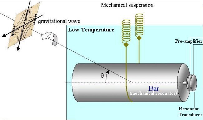
Figure 10t GW Detector
| Gravitational wave have never been observed because of low radiation power and weak interaction strength. A rod about 1 meter long spun at the verge of breaking would radiate perhaps 10-30 erg/sec. The cross section for the interaction between gravitational wave of ~ 104 cycles and an ammonia molecule is roughly 10-60 cm2. Figure 10t is the schematics of a gravitational wave bar detector. The impinging gravitational wave excites the fundamental longitudinal resonance (at ~ 1000 Hz) of the bar, kept at low temperatures. The induced vibration of the bar end face is amplified mechanically by the resonant |
| transducer, which also converts the signal into an
electromagnetic one. The signal is then amplified and acquired (see
Figure 10t). It is suggested that large-scale astronomical motions of
matter could generate appreciable gravitational energy flux.
Figure 10u GW from Binary Pulsars
|
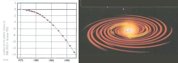
| The binary pulsar PSR1913+16 was discovered in 1975. This system consists of two compact neutron stars orbiting each other with a maximum separation of only one solar radius. The rapid motion means that the orbital period of this system should decrease on a much shorter time scale because of the emission of a strong gravitational wave. The change predicted by general relativity is in excellent |
agreement with observations as shown in Figure 10u. Thus,
the observation indirectly confirms the phenomena of gravitational
radiation.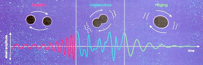 Figure 10v Black Hole Merger
|
| Figure 10v illustrates the merger of two orbiting black holes. Initially, the gravitational signals from such an event would show oscillation with increasing amplitude and decreasing wavelength as the black holes spiral toward each other. A chaotic pattern of gravitational waves may be given off at the moment of merger. Finally, the resultant single black hole is expected to |
| "ring", creating waves with diminished amplitude. This
event will emit no x-ray burst, not even a flash of light. |
Gravitational waves may be viewed as coherent states of many gravitons,
much like the electromagnetic waves are coherent states of photons. Since
gravitational wave has evaded detection for over 50 years, it seems even
harder to find the individual gravitons. However, it is suggested that in
high-energy colliders such as the LHC, it is possible to produce gravitons,
which can then disappear into the extra dimensions. This would lead to a ‘missing energy’ signature, with
unbalanced events. Such signatures are routinely used in particle
experiments to detect the production of neutrinos (difficult to detect). The
exchange of gravitons in the extra dimensions would also affect the dynamics
of other scattering processes.
A leading cosmological model, known as inflation, predicts that our universe is just one part of a greater multiverse and that
our Big Bang may have been one of many. In this model, our universe expanded
extremely rapidly during the period of 10-35-10-32
second after the Big Bang.
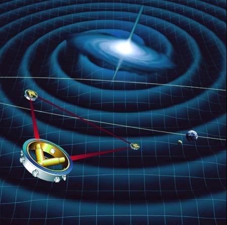
Figure 10w LISA
Another model, rooted in string theory, envisions a scenario in which the Big Bang occurred as a
| result of the collision between two parallel universes floating in higher dimensional space. Each of these models predicts a specific pattern of gravitational waves emitted from the Big Bang. NASA and ESA plan to launch the Laser Interferometer Space Antenna (LISA) to detect gravitational wave by 2013. It consists of three satellites orbiting the sun (Figure 10w). They will be linked by three laser beams, forming a triangle of light. They are designed to detect a change in their spacing as small as 1/10 the diameter of an atom. With such sensitivity LISA might be able to detect gravitational waves created immediately after the birth of the cosmos. It offers a chance to select between the contesting cosmological models, and also provides an opportunity to test the string theory. |
Schwarzschild's Solution and Black Hole
The equations of gravitational field can be solved exactly for the case
of a centrally symmetric field in vacuum with mass M at the center. In terms
of spherical coordinates and ct, the space-time metric has the form:
ds2 = - (1 - 2GM/c2r) c2dt2 + dr2
/ (1 - 2GM/c2r) + r2 (sin2![]() d
d![]() 2
+ d
2
+ d![]() 2)
---------- (13)
2)
---------- (13)
This is known as the Schwarzschild solution. It is a useful example for
illustrating the effect of gravity in general relativity:
- As r
 ,
the space-time metric reduces to the expression for flat space-time:
,
the space-time metric reduces to the expression for flat space-time:
ds2 = - c2dt2 + dr2 + r2 (sin2 d2
+ d2)
---------- (14)
d2
+ d2)
---------- (14)
- At the non-relativistic limit where v2/c2 << 1,
an expression for the space-time metric can be derived from classical
mechanics:
ds2 = - (1 + 2V/c2) c2dt2 + dr2 + r2 (sin2 d2
+ d2)
d2
+ d2)
where V is the gravitational potential.
Comparing with the space-time metric g44 in Eq.(13) in the region where r > 2GM / c2, the Newton's law of gravitation: V = - GM / r is recovered from general relativity. Thus, at the non-relativistic limit only the time dilation effect (relating to g44) is important. The effect of spatial curvature (relating to g11) is negligible at this limit.
- At the distance where r = rs = 2GM/c2, the
escape velocity ve = (2GM/r)1/2 = c. It implies that
even light cannot escape the grip of gravity at this point. This is
Schwarzschild radius separating the black hole from the rest of the world.
- A black hole can form only when the Schwarzschild radius rs is outside the central object. For the Earth, and the Sun, rs is well inside the physical boundary (rs for the Earth is about 1 cm and for the Sun is about 3 km). Even the neutron star (with similar mass to the Sun) has a physical radius of about 10 km. Only collapsing stars or galactic center have the necessary condition to form a black hole. Figure 09a is an embedding diagram (Figure 09b) of a black hole. The two dimensional circles are the projection of three dimensional spheres - the
Figure 09a Black Hole
hyperspace. The vertical axis denotes the "stretch" of space in the radial direction. The slope of the curve can be considered as representing the curvature of the space.
- Gravitational redshift is generated as the photons loss energy in overcoming the pull of the gravitational field (see Figure 09c). For the case of a black hole, the shifted wavelength is computed by the formula:
 =
o
/ (1 - rs/r)1/2
=
o
/ (1 - rs/r)1/2
At the Schwarzschild radius rs, the redshift becomes infinity. This is the effect that makes light invisible at rs.Figure 09c Redshift
- The gravitational field also induces time dilation as experienced by a
far away stationary observer. It is in a similar form:
T = To / (1 - rs/r)1/2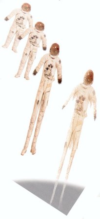
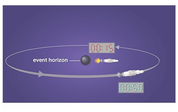
Figure 09d Tidal Force Figure 09e Time Dilationwhere To is the time interval recorded by an observer plunging toward the black hole and T is the corresponding time perceived by a stationary observer. Thus, for the stationary observer it takes an infinite long interval for the other
observer approaching the Schwarzschild radius rs. However, the adventurer is not aware this curious effect on the time interval. His journey may be interrupted only by the tidal force, which is much more ferocious for black hole with smaller size (the tidal force at rs is equal to  2GM / rs3 =
c6/(2GM)2, the + and - signs represent the
stretch and squeeze parallel and perpendicular to the radial direction
respectively, see Figure 09d). Figure 09e shows the time dilation for
a space traveler located at a distance of 1.1 rs from the
center of a black hole.
2GM / rs3 =
c6/(2GM)2, the + and - signs represent the
stretch and squeeze parallel and perpendicular to the radial direction
respectively, see Figure 09d). Figure 09e shows the time dilation for
a space traveler located at a distance of 1.1 rs from the
center of a black hole. 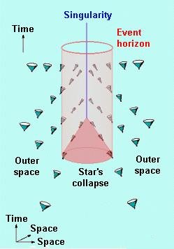
- Inside rs, all matter must fall towards the center, even light, which keeps coming from outside (but cannot get out from inside). After a finite time the inward falling object will end up at r = 0, where the density of matter is infinite. The metric g44 changes sign inside the black hole, i.e., time has become just another dimension of space. It is suggested such change has the effect of smoothly rounded off the singularity at r = 0. There is speculation that quantum effect will remove the singularity; it might provide a gateway leading to another universe. Figure 09f shows a collapsing star, and the behavior of light near and inside the black hole. The effect of the black hole on light is indicated by the direction of the light cone. It shows that far away from the black hole the light cone points to all directions around. The directions are tilted toward the black hole as it moves closer. At the event horizon it cannot escape to outside. The directions of the cone only point to the center once inside the black hole, there is no turning back.
Figure 09f Black Hole, Inside
- White holes are similar to black holes except white holes are ejecting matter while black holes are absorbing matter. The existence of white holes is implied by the negative square root solution to the Schwarzchild metric. In particular, if we define the proper time d
 to be the time associated with the moving frame, in which the spatial
variation vanishes (co-moving objects are stationary in that frame),
then
to be the time associated with the moving frame, in which the spatial
variation vanishes (co-moving objects are stationary in that frame),
then Figure 09g White Hole
c2 d  2
= -ds2 = -g44 c2 dt2
2
= -ds2 = -g44 c2 dt2
where g44 is negative according to the convention. Thus,d
= ± (-g44)1/2 dt
where the positive sign corresponds to the black hole solution while the solution with negative sign is interpreted as the white hole with time running backward. Figure 09g depicts an embedding diagram of a white hole, which is just a black hole turned upside down to give an illusion that matter is spilling out instead of pouring in.
- The space-time metric for a static wormhole (also known as the
Einstein-Rosen Bridge) can be expressed in the form:
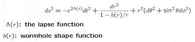
---------- (15a)
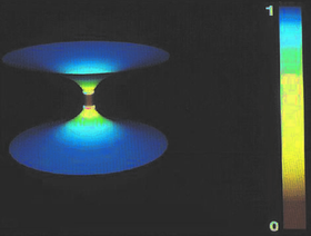
The lapse function defines the proper time between consecutive layers of spatial hyper-surfaces; while the shape function determines the shape of the worm hole. The shape function takes on a very simple form for the case of the Schwarzschild's metric, i.e., b(r) = 2GM / c2 = rs. The throat of the wormhole is located at r = b(r) = rs in this case. Figure 09h is a computer generated embedding diagram of a blackhole, a wormhole, and a whitehole. The surface of the diagram measures the curvature of space. Color scale represents rate at which idealized clocks measure time; red is slow, blue fast. Figure 09h Wormhole
Another way to conceptualize a wormhole topology is to have the spatial part of the space-time metric in Eq.(15a) imbedded in a flat hyperspace with the extra-dimension denoted by W: dl2 = dW2 + dr2 + r2 (sin2
d2)
= dr2 / (1 - rs/r) + r2 (sin2
d2)
---------- (15b)
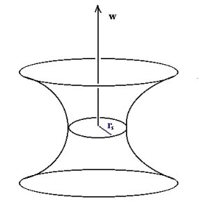
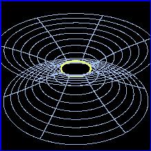
Figure 09i Worm- hole in Hyperspace Figure 09j Worm- hole Throat
Eq.(15b) can be used to equate dW =
(r/rs - 1)-1/2dr. Integration of the equation
gives W2 = 4rs(r - rs), which is a
parabola function with vertex at W = 0, r = rs. Sweeping
the curve around the W axis to include all values of
from 0 to 2
results in a paraboloid surface as shown in Figure 09i. Inside the wormhole, g11 and g44 change sign as shown in Eq.(13). The region becomes space-like, which means two events cannot be linked unless the signal propagates with greater than light speed. This peculiar property is also related to the instability of the wormhole. However it is suggested that if there is a large amount of negative mass/energy -m (in the forms of a thin spherical shell, which appears in the embedding diagram as the yellow circle as shown in Figure 09j) to sustain the structure, then creation of a wormhole may become feasible. The negative mass ensures that the throat of
the wormhole lies outside the horizon (since the new event horizon is now 2(M-m)G/c2), so that travelers can pass through it, while the positive surface pressure of such exotic material would prevent the wormhole from collapsing. This would allow for shortcut in space travel within the wormhole between two distant points (see Figure 09k), or for the possibility of time travel courtesy of LHC (Figure 09l).
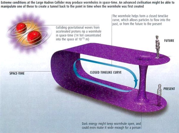
Figure 09l Time Travel
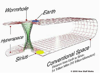
Figure 09k Space Travel
Kerr's Solution and Rotating Black Hole
The space-time metric generated by a rotating mass M with angular velocity
![]() was found by Roy Kerr in
1963:
was found by Roy Kerr in
1963:
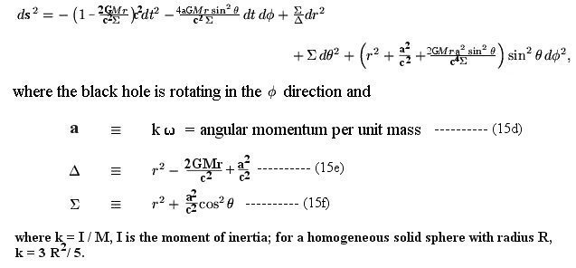 |
---------- (15c) |
- At r , the Kerr's
metric reduces to the one for flat space-time (same as Eq.(14)):
ds2 = - c2dt2 + dr2 + r2 (sin2 d2
+ d2) ----------
(15g)
- The Kerr's metric reduces to the Schwarzschild's metric in Eq.(13)
naturally when a = 0, i.e., with no rotation.
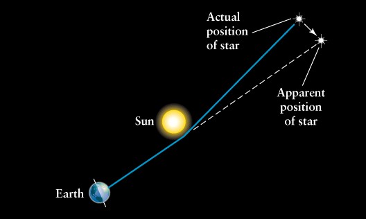
Figure 09m Bending of Light
- The trajectory of light ray can be computed from the equation of motion Eq.(12b), or from the equation of energy conservation. It was shown theoretically that light ray is deflected by gravitational field, e.g., binding of distant star light near the sun (see Figure 09m). This prediction was first confirmed by Sir Arthur Eddington's 1919 solar eclipse expeditions. If the light ray comes close enough to a dense object, the path will be bent so much that it runs around in a circle. For non-rotating black hole such special trajectory occurs at r = 3rs/2 = 3GM/c2. The sphere with such a radius is
called the photon sphere. However, the orbit is unstable; it can be disrupted with very small perturbation. Mathematically, such precarious orbit is defined by d2r / d 2
= 0. It is from this formula that the radius of the photon sphere is
deduced. There are two photon spheres for the rotating black hole - an outer one for light ray traveling in a direction opposite to the spin of the black, and an inner one for co-rotating light ray.
- As r descends further toward the center, the space-time metric g44
(or gtt) vanishes at
r = [GM + (G2M2 - a2c2cos2)1/2]
/ c2 ---------- (15i)
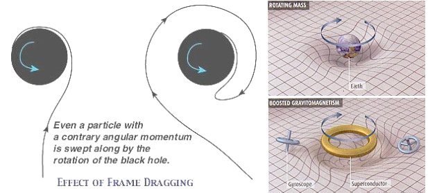
Figure 09n Frame Dragging
This is called static limit. It can be intuitively characterized as the region where the rotation of the space-time is dragged along with the velocity of light. Within this region, space-time is warped in such a way that no observer can maintain him/herself in a non-rotating orbit, but is forced to become co-rotating (Figure 09n). The surface of this region is elliptical with its major axis at =
/2 (the equator), and r =
2GM / c2 (= the non- rotating Schwarzschild's radius). The minor axis is in the directions of = 0, and
(the poles), and r = [GM
+ (G2M2 - a2c2)1/2]
/ c2 (see Figure 09o).
It is found in 2006 that a spinning superconductor generates a much larger drag than that from a regular rotating mass. The effect is attributed to some sort of "gravitomagnetism" (Figure 09n, no relation to electromagnetism) produced by massive gravitons similar to the Meissner effect produced by massive photons. The discovery may fulfill the "anti-gravity device" perpetrated by science fictions.
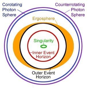
Figure 09o Kerr's Solution
- A rotating black hole is very different from a Schwarzschild black hole in that the spin of the black will cause the creation of two event horizons instead of just one (see Figure 09o). The outer event horizon occurs at
r+ = [GM + (G2M2 - a2c2)1/2] / c2 ---------- (15j)
The inner horizon (sometimes called the Cauchy horizon) is located at
r- = [GM - (G2M2 - a2c2)1/2] / c2 ---------- (15k)The Ergosphere is the region between the static limit and the outer event horizon. Since this region is outside the event horizon, particles falling within the ergosphere may escape the black hole extracting its spin energy in the process. The separation between the two horizons is 2 (G2M2 - a2c2)1/2 / c2. For a = 0, r- =0, hence for a non-rotating black hole, the inner event horizon can be considered as fallen into the center. As the spin increases, the two horizons move toward each other and merge at r = GM / c2 when a / c = GM / c2. In case a / c > GM / c2, there will be no event horizon, the black hole becomes a "naked singularity", i.e., it is not covered by an event horizon.
Note 1: The only physical part of a black hole is the singularity. The static limit, and event horizon are not physical barrier; they only mark the imaginary boundaries between types of space.
Note 2: A proposal in 2007 suggests that naked black hole should be detectable via the "gravitational lenses" effect. Existing telescopes should have sufficient spatial resolution to spot naked singularities in the center of the Milky Way.
- A rotating black hole is very different from a Schwarzschild black hole in that the spin of the black will cause the creation of two event horizons instead of just one (see Figure 09o). The outer event horizon occurs at
- As r
 , a singularity
develops in the form of a ring at the equator (see Figure 09p), where
/2, and cos
0 in such a way that r >
(a / c) cos. The Kerr's
metric then becomes:
, a singularity
develops in the form of a ring at the equator (see Figure 09p), where
/2, and cos
0 in such a way that r >
(a / c) cos. The Kerr's
metric then becomes:
ds2 = - (1 - 2GM / c2r) c2dt2 + (2GMa / c2r) dt d
+ (a2/c2) (1 + 2GM / c2r) d2
---------- (15n)
The severity of the singularity depends on the angular momentum per unit mass a. If a is sufficiently large it would be very mild; on the other hand it becomes a point singularity at the limit a 0. Away from the ring of
singularity in the region where r ~ 0, the Kerr's metric has the form:
ds2 = - c2dt2 + cos2
dr2 + (a2/c2) (cos2
d2 + sin2
d2) ----------
(15o)
Interesting theoretical physics can take place around this ring singularity. Since 1 g11 =
cos2 in Eq.(15o),
the spatial curvature is negative, which acts like a repulsive force. One
consequence is that nothing can actually fall into this region unless
approaching in a trajectroy along the ring's side. Any other angle and the
negative spatial curvature actually produces an antigravity field that repels
matter. It could be the mechanism that produces the jets observed in many
black holes.
g11 =
cos2 in Eq.(15o),
the spatial curvature is negative, which acts like a repulsive force. One
consequence is that nothing can actually fall into this region unless
approaching in a trajectroy along the ring's side. Any other angle and the
negative spatial curvature actually produces an antigravity field that repels
matter. It could be the mechanism that produces the jets observed in many
black holes.
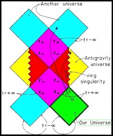
Figure 09p Penrose Diagram
- The Penrose diagram in Figure 09p summarizes all regions of space-time associated with a rotating black hole. A penrose diagram is not meant to accurately portray distances, it describes only the causal structure. Only radial and time directions are represented while angular directions are suppressed. The units of space and time are scaled in such a way that any object moving at the speed of light will follow a path at an angle of 45º to the vertical. All possible paths for physical objects must stay closer than 45º to the vertical. The green diamond represents our entire Universe over its entire history and destiny, from the infinite past to the infinite future (it takes an infinite amount of time to cross the outer event horizon from the view point of a distant observer). The purple diamond is the region between the outer and inner event horizons, where everything plunges inward. The red area denotes the space between the inner event horizon and the ring singularity, where the space-time re-acquires its normal characteristic with rising curvature toward the ring singularity. The other half in yellow is the region
inside the ring singularity, where the gravity becomes repulsive. The blue diamonds can be interpreted as another universes or another part in our own universe. This concept is similar to the wormhole in the Schwarzchild's solution. 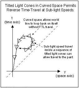
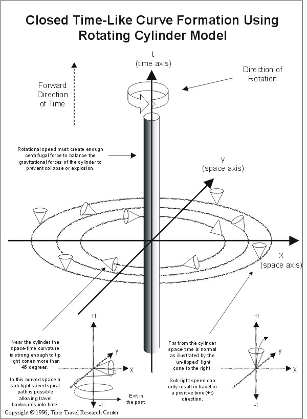
As depicted in the Penrose diagram, the space-time metric g11 (or grr) changes sign when crossing over the first event horizon, and then reverses back again at crossing over the second horizon. Thus between the two horizons, space and time exchange places. Instead of time always moving inexorably onward, the radial dimension of space moves inexorably inward to the Cauchy horizon. After that the Kerr solution predicts a second reversal, which implies no more plunging inward. In this strange region inside the Cauchy horizon the observer can, by selecting a particular orbit around the ring singularity, travel backwards in time and meet himself, in violation of the principle of causality (cause must precede effect). It is surmised that a closed time-like curve (CTC, Figure 09q) to loop back to the past is possible in a heavily curved space-time (Line A in Figure 09p). Another possibility admitted by the equations for the observer in the central region is to plunge through the hole in the ring into an antigravity region (Line B). Or he can Figure 09q Closed Time-like Curve (CTC)
travel through two further horizons (or more properly anti-horizons), to emerge at coordinate time t = –  into some other universe (Line C). These exotic properties of rotating
black holes have inspired several science fiction stories.
into some other universe (Line C). These exotic properties of rotating
black holes have inspired several science fiction stories.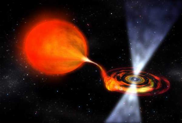
Figure 09ra Disk and Jets
- A more realistic rotating black hole would have an accretion disk around the equator and a pair of jets ejecting along the poles. An accretion disk is matter that is drawn to the black hole. As matter is gradually pulled into the center, it gains speed and energy. It can be heated to temperatures as high as 3 billion K by internal friction, and emit energetic radiation such as gamma rays. Some of the particles that has funneled into the disk-shaped torus by the hole's spin and magnetic fields, can escape the black hole in the form of high speed jets along the poles (Figure 09ra).
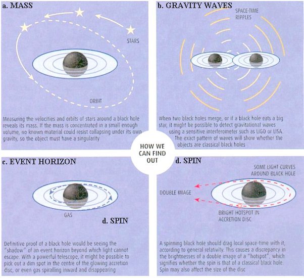
Figure 09rb Black Hole Detections
- Black Holes are very difficult to detect because they are black. It would be a definitive proof of their existence if we can see the "shadow" in the form of a dim spot in the centre of the glowing accretion disc (Diagram c in Figure 09rb). Most of the circumstantial evidences come from observing high velocity objects moving tightly in small space as shown in Diagram a, Figure 09rb. Other evidences involve detecting gravity waves from merging black hole(s) or the double image from a spinning black hole (see Diagram b and d in Figure 09rb), which throws out huge jets of debris to advertise its presence. The final answer to whether our black hole ideas are correct would be sending a probe to a nearby candidate and have it transmit data as it makes its final plunge.
Since most collapsing massive objects would have some initial angular
momentum, the Kerr's metric seems to be a more realistic representation for
the black hole space-time. However, it is argued that the collapsing object
would lost its rotational energy in the form of gravitational wave and ends up in a perfect spheroidal shape. Whichever to be the case,
followings are some comments on the Kerr's metric and its modification to the
Schwarzschild's black hole:
A Scenario for Time Travel
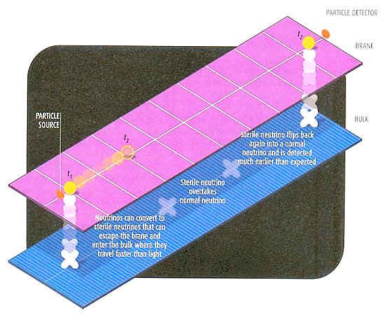
| Recently in 2006, a scenario for time travel has been proposed without relying on rotating black holes or exotic wormhole tunnels. The idea is based heavily on the Superstring theory, according to some versions of which, our universe is a four-dimensional membrane or "brane" embedded in a higher-dimensional hyperspace called the bulk. Almost all matter and force-carrying particles are trapped on the 3-D brane, where they are contrained to travel at the speed of light or lower. However, sterile neutrinos and gravitons are particles that can access the hidden dimensions and travel faster than light (Figure 09s). From some view points or frames of reference, this is equivalent to time travel (see Figure 05, event 4). |
| The main ingredients of this theory are summarized in the
followings: Figure 09s Time Travel |
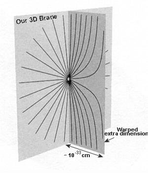
- For many years, physicists believed that extra dimensions were acceptable, but only if they were finite in size, either curled up or bounded between branes. An infinite extra dimension was supposed to destablilize everything around us. It is now known that infinite extra dimension from a single brane (like our 3D brane) is possible if that extra dimension is heavily warped so that the gravitons are localized near the brane in a small region no more than the Planck length scale of 10-33 cm (see Figure 09t).
- Thus, instead of the requirement for a heavily curved space-time in our 3D universe, or a folding one such as shown in Figure 09k, a model can be conceived such that the extra dimension in the bulk is seriously warped. It is found that the extra dimensions can be distorted by exotic matter in such a way that anything moving through the bulk can travel faster than the speed of light. Such off-brane short cuts can appear as "closed time-like curves" (CTC) as shown in Figure 09q.
- This has dramatic consequences for inhabitants stuck on the 3D universe. To them, any entity that takes a short cut through the bulk appears to vanish and then pops up again at some point far sooner than it could have had it kept to the 3D universe, and in some other frames of reference, it has travelled backward in time (see Figure 05, event 4).
- However, according to the Superstring theory, only closed strings such as the sterile neutrinos and gravitons can wander into the bulk. We may not be able to do time travel ourselves, but we can study time travel experimentally by manipulating these particles. The problem is that no one has ever spotted a graviton or a sterile neutrino.
- Nevertheless, experiment to test time travel has been proposed via the mechanism of neutrino oscillation, which could change ordinary neutrinos into sterile neutrinos and vice versa. The odds of this happening increase whenever the density of the material the neutrinos are travelling through changes abruptly. Thus, it is suggested that a beam of ordinary neutrinos would be sent through the Earth, from South Pole to a detector located at the equator. Some of them flipped into sterile neutrinos going through the bulk and emerge as ordinary neturino (via another flipping), which may appear as moving at greater than light speed or arrived before setting off.
- Critics point out that even if future technology can manipulate sterile neutrino in the next 50 years or so, the problem with the hypothetical exotic matter (to produce the warped space-time) is only shifted from our universe to unknown dimensions. Concealing the problem in the bulk is little better than a scenario in which it is out in the open. However, if the experiment is successful, it will verify many conjectures such as higher dimensions, some versions of the Superstring theory, sterile neutrinos, exotic matter in higher dimensions, and time travel albeit only for sterile neutrinos and gravitons.
|
|
| Figure 09t Extra Dimension
|
Hawking Radiation
According to Stephen Hawking himself, an inspiration came to him before
going to bed one evening in 1970 (getting into bed is a rather slow process with
his disability). He suddenly realized that since nothing can escape from a black
hole, the area of
the event horizon might stay the same or increase with time but it could never
decrease. In fact, the area would increase whenever matter or radiation fell
into the black hole. This non-decreasing behavior of a black hole's area was
very reminiscent to that of entropy, which measures the degree of disorder in a system. One can create order out of
disorder, but that requires expenditure of effort or energy such that there is
an overall increase in disorder. In simple mathematical terms these statements
can be expressed in differential forms as:
m dm = k dA ---------- (16a) for the black hole (since A
![]() rs2
rs2
![]() m2 from the
Schwarzschild's solution),
m2 from the
Schwarzschild's solution),
where m is the mass of the black hole, A is the area of the event horizon, and k
is a proportional constant;
dE = T dS ---------- (16b) for the entropy,
where E is the energy, T is the temperature, and S is the entropy.
Since mass and energy are equivalent, we can equate Eqs.(16a) and (16b) to
obtain:
dS = K dA / ( m T ) ---------- (16c)
where K is a new proportional constant. This equation implies that the area of
the event horizon A is a measure of the entropy S of the black hole. Furthermore,
the black hole is associated with a temperature T, and should emits radiation as
any hot body. Thus, the black hole is not completely closed to the universe
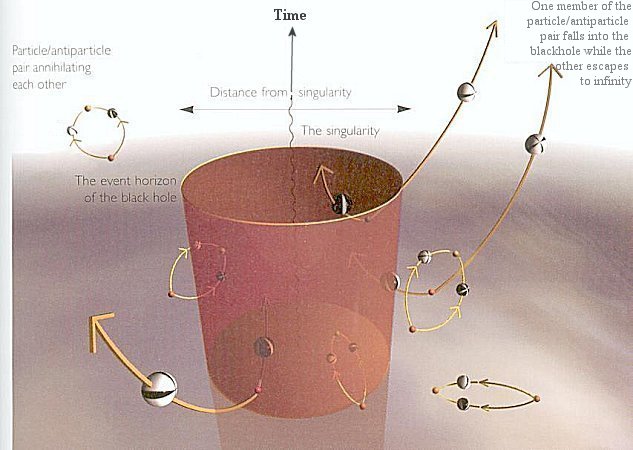
outside. It turns out that vacuum fluctuations at the edge of
| the event horizon may allow one member of the virtual particle / anti-particle pair to fall inside with negative energy; while the other escapes as a real particle with a positive energy according to the law of energy conservation. This is known as Hawking radiation (see Figure 09u); it is the first successful attempt to combine general relativity and quantum theory. The flow of negative energy (or mass) into the black hole would reduce its |
| mass. As the black hole loses mass, the area of its event
horizon gets smaller, but this decrease in the entropy of the black hole is
more than compensated for by the entropy of the emitted radiation, so that
the second law of thermodynamics is never violated. If we demand that in Eq.(16c)
Figure 09u Hawking Radiation
Figure 09v Blackhole Evaporation
|
dS ![]() dA as stated
originally (actually, it can be shown that S = (kBc3/4G
dA as stated
originally (actually, it can be shown that S = (kBc3/4G![]() )
x A), then T
)
x A), then T ![]() 1 / m, and the
rate of radiation L can be expressed as L
1 / m, and the
rate of radiation L can be expressed as L
![]() rs2T4
rs2T4
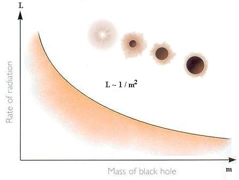
![]() 1 / m2. Therefore,
as the black hole loses mass, its temperature and rate of emission increase,
then it lose mass even more quickly (Figure 09v). What happens when the mass of
the black hole eventually becomes extremely small is not quite clear, but the
most reasonable guess is that it would disappear completely in a tremendous
final burst of emission.
1 / m2. Therefore,
as the black hole loses mass, its temperature and rate of emission increase,
then it lose mass even more quickly (Figure 09v). What happens when the mass of
the black hole eventually becomes extremely small is not quite clear, but the
most reasonable guess is that it would disappear completely in a tremendous
final burst of emission.
It can be shown that the temperature T associated with the thermal radiation for
a black hole is:
T = 0.6 x 10⁻⁷ msun / m (in degrees Kelvin)
where msun is the mass of the Sun. If the Sun is reduced to a black
hole, its temperature would be just about 10-7 oK. On the
other hand, there might be primordial black holes with a very much smaller mass
that were made by the collapse of irregularities in the very early stages of the
universe. Those with masses greater 1015 gm could have survived to
the present day. They would have the size of a proton (~ 10-13cm) and
a temperature of 1011 oK. At this temperature they would
emit photons, neutrinos, and gravitons in profusion; they would radiate
thermally at an ever increasing rate, and sending out X rays and gamma rays to
be discovered. The lifetime of a black hole is roughly equal to
![]() = m / L = 10-35 m3
year, where m is in gm. This makes an ordinary mass black hole (m ~ 2x1033
gm for the Sun) live for a long time and its radiation unobservable.
= m / L = 10-35 m3
year, where m is in gm. This makes an ordinary mass black hole (m ~ 2x1033
gm for the Sun) live for a long time and its radiation unobservable.
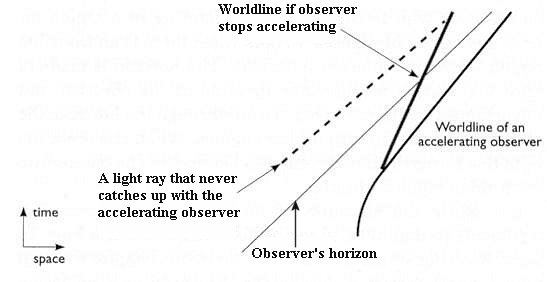
Figure 09w Event Horizon of an Accelerating Observer
| This phenomenon of Hawking radiation also occurs in the event horizon created by an accelerating observer. Figure 09w shows that light ray emitted at certain distance can never catch up with the observer and thus an event horizon exists beyond which the observer cannot communicate. Theoretical arguement suggests that even in empty space, the observer will be able to detect radiation from the event horizon. A simple formula is derived to express the relationship between the acceleration a and the temperature T: |
| T = a ( |
- According to general relativity anything that crosses the event horizon is trapped inside forever lost to the outside world.
- In spite of his own discovery of Hawking radiation, which can return matter-energy back to the outside world, Hawking himself insists that information would be destroyed by the black hole.
- Since entropy is related to information, the loss of information would violate the second law of thermodynamics, which holds that entropy would neither decrease nor disappear. Thus, the critics argue that nature may scramble information but never destroys it.
- To resolve the dispute, 't Hooft and Susskind proposed the "Principle of
Black Hole Complementarity" in which both sides are correct. For the outside
observer, matter (the elephant in Figure 09x) would be reduced to thermal
radiation
at the event horizon (as it takes an infinite time for the elephant to cross such boundary according to observer a) and returns as scrambled information. For an observer crosses the event horizon into the black hole, nothing untoward happens until the tidal force takes over ... information is forever lost. Figure 09x Black Hole Information Paradox
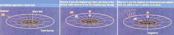
- Such duality is further likened to a hologram located on some surface. There are two possible ways to interpret the hologram: one view corresponds to that for the outside observer a in Figure 09x; while the other represents the perception from observer b falling into the black hole.
Black hole and information:
| Meanwhile, other research in superstring theory finds the black hole to be a "fuzzball" (Figure 09y). The modified black hole does not possess a sharp event horizon; information can be stored in the strings and imprinted on outgoing Hawking radiation. Models of black holes from superstring theory also cast doubt on the idea of the singularity (at the center of the black hole). Yet another scheme suggests that information might leak out by means of quantum teleportation between the entangled pair of virtual particles (one of which has escaped while the other is trapped inside the black hole). However in the theory of loop quantum gravity, it has been shown that the information trapped in a black hole will be unable to escape via Hawking radiation. But it will survive, eventually rejoining the rest of the universe when the black hole evaporates. |
| Figure 09y Fuzzball
|
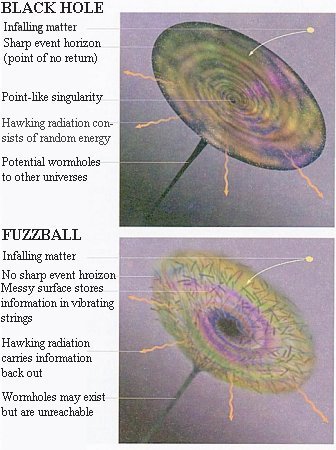
Standard Cosmology
Another example that offers exact solution is the homogeneous and isotropic space filled with pressure-less dust. It is applicable to the case of the cosmic expansion, if each dust point presents a galaxy. Universes of this type are variously known as Friedman universes, Friedman-Robertson-Walker universes, ... etc.
- The space-time interval is associated with the Robertson-Walker metric. It
has three forms depending on the curvature of the 3
dimensional space:
ds2 = R(t)2 (dw2 + s2 (d2
+ sin2 d2))
- c2dt2 ---------- (17)
where s = sin(k1/2 w) / k1/2, and R(t) is called the scale factor.
For flat space with zero curvature, k = 0, and s = w.
For closed space with positive curvature, k = +1, s = sin(w), where w ranges from 0 to 2.
For open space with negative curvature, k = -1, s = sinh(w), where w ranges from 0 to infinity.
- In term of the Robertson-Walker metric and with the energy-momentum tensor
T00 =
 , the
gravitational field equation becomes:
, the
gravitational field equation becomes:
(dR/dt)2 + kc2 = 8GR2
/ 3 ---------- (18a)
which can be re-arranged into the form:
k2 c2 = H2 R2 ( - 1) ---------- (18b)
where H(t) = (dR/dt) / R is the Hubble's parameter, =
/
c, and
c = (3 H2)
/ (8G) is the critical density,
which corresponds to the total energy density for a flat universe. Eq.(18b)
shows that
for flat space,=
c,
= 1, and k = 0;
for closed space, >
c,
> 1, and k = +1;
for open space, <
c,
< 1, and k = -1.
- More generally, when several types of matter coexist in the universe, the
following consistency relation must be satisfied:
 jj
+ k = 1
jj
+ k = 1
where the sum is over the various types of matter andk = - kc2/(R0H0)2
with the subscript "0" standing for present quantities. Present cosmological
observations yield:
b ~ 0.04 for
brayons (ordinary visible and nonluminous matter),
d ~ 0.26 for
exotic dark matter,
 ~ 0.7 for dark energy,
 ~ 5 x 10⁻⁵ for photons (radiation), and
k = 0.
- If we choose = M / (4R3/3)
---------- (18c)
where M may be interpreted as the total mass of the universe, Eq.(18a) becomes:
(dR/dt)2 + kc2 = 2GM / R ---------- (18d)
The solution for this equation is:
for k = 0, R = (9GM/2)1/3 t2/3, t = 2/3H ---------- (19a)
for k = +1, R = Ro (1 - cos(µ)), ct = Ro (µ - sin(µ)) ---------- (19b)
where Ro = GM / c2, and µ is defined by c dt = R(µ) dµ.
for k = -1, R = Ro (cosh(µ) - 1), ct = Ro (sinh(µ) - µ) ---------- (19c)
For the radiation (relativistic matter) dominated universe, the radiation pressure p =/3. Starting
from the thermodynamic relation dU = -pdV, where U =
V, and V is the volume of the
system (the universe in this case), it can be shown that
 1/R4, Eq.(18a) (for
the case k = 0) becomes dR/dt
1/R, the solution for
which is R t½.
1/R4, Eq.(18a) (for
the case k = 0) becomes dR/dt
1/R, the solution for
which is R t½.
Incidentally, since the temperature T is related to the energy density as
T4, thus T
1/R.
- The red shift caused by the cosmic expansion can be expression in terms of
the scale factor R [see Figure 09z, which shows the red shift of the Balmer
series of the hydrogen line spectra (dark lines, denoted by H
 ,
...) superimposed on the continuous spectra (colored), the arrows indicate the
direction of increasing values for the corresponding variables]:
,
...) superimposed on the continuous spectra (colored), the arrows indicate the
direction of increasing values for the corresponding variables]:
z =1 /
2 - 1 = R(t2)
/ R(t1) - 1 ---------- (19d)
Figure 09z Cosmic Red Shift
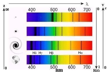
where t2 denotes the current epoch, 2 is the
original wavelength (as measured on Earth),
1 is the
wavelength of a spectral line that was emitted at time t1 (red
shifted) in the distant past, R(t2) is often taken to be 1 for
convenience, then R(t1) is less than 1 in the past and is often
just denoted as R(t). The quantity (z + 1) can be considered as the amount
of stretching during the intervening time for the light to travel from
there to here. It is a curious relativistic effect that the velocity and
distance remain finite approaching the velocity of light and the event
horizon respectively even though the amount of stretching becomes infinity. The relativistic expression for z+1 (In terms of the recession velocity v) is: z + 1 = [(1+ v/c) / (1- v/c)]1/2.
- From the observed value of the Hubble constant Ho = 71 km/sec-Mpc for the
current epoch, and by substituting the speed of light c for v in the Hubble's
law: v = Ho d, it follows that the rate of cosmic expansion would be
exceeding the
speed of light beyond a distance dh = c/Ho = 1.27x1028 cm. However, there is no contradiction, because special relativity states that no signal can propagate faster than the speed of light, but the expansion of the universe cannot be used to propagate a signal although it can move with superluminal speed. We will not be able to see this region anyway because the event horizon is located right at the boundary (Figure 10b), if we take the Hubble time T = 1/Ho = 13.7 billion years (from WMAP data) to be the the age of the observable universe. Figure 10b illustrates the Hubble's law with a space-time diagram. Consideration of kinematics alone shows that a subtle inconsistency is hidden in the original form of the formula.
Figure 10a Event Horizon
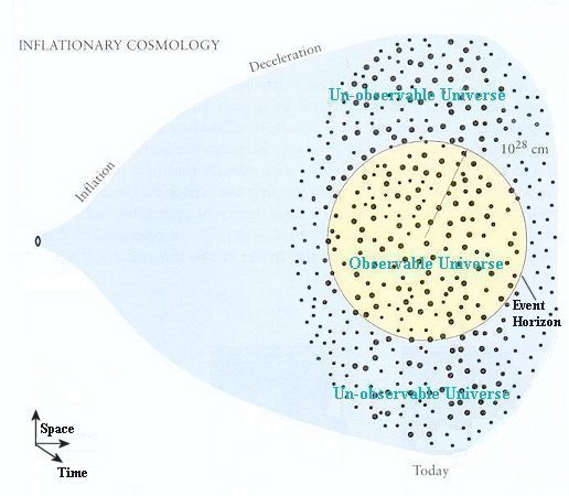
Figure 10b Space-time Diagram
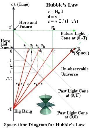
Since the Hubble's law is an empirical formula, so the distance should be referred to the lookback distances, which is measured some time in the past. Analysis of the space-time diagram shows that the formula is actually related to the comoving distance d, which can be considered as measured by a ruler moving
| together with our frame of reference. In Figure 10b, all the objects emanated from the Big Bang are represented by the red solid lines with different velocity v. They are straight lines because the Hubble's law assumes constant velocity in cosmic expansion without considering the effects of inflation, gravitational retardation, and dark energy acceleration. The corres-ponding lookback distance is marked as s1, s2, s3, ... until the lookback event horizon sh for object moving with the speed of light. The comoving distance in the |
| current epoch corresponding to different v is labeled by d1, d2, d3, ... until the event horizon dh. The past light cone (in black solid line, the cone is made by rotating |
this line around the time axis as shown by the small insert) indicates light signal from objects with different rate of recession reaching the observer at "Here and Now". It can be shown that d = vT = s (1+v/c). For Hubble's original data in 1929 s ~ 1 Mpc and v ~ 500 km/s, the difference between the two definitions of distance is about 0.001 Mpc.
Figure 10c Cosmic Distance
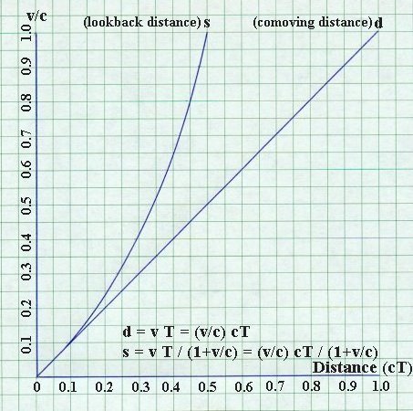
Figure 10d Quasar Data
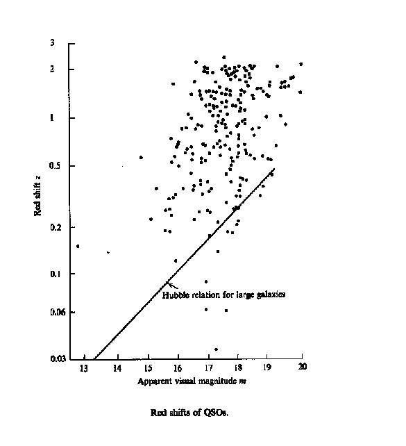
The difference for higher red-shifted objects would be considerably more (~ 10% for the furthest data point),
and up to cT/2 for v = c (Figure 10c). Thus, the original Hubble's law (associated
with observational data) in the form s = vT is valid only for v << c. The
green lines in Figure 10b depict the situation at a future time T'; it shows
the expanding lookback event horizon s'h. The unobservable universe
occupies the region outside the future light cone at the Big Bang.
Quasars possess
very high red shift up to z = 2.5 corresponding to v/c = 0.85. Figure 10d
shows the observational data relating red shift to the apparent visual
magnitude. The red shift can be translated to the recession velocity by the
formula v/c = [(z+1)2-1]/[(z+1)2+1], while the apparent
visual magnitude
m can be expressed in terms of the absolute magnitude M and the lookback
distance s (in cm) as m = M - 97.5 + 5xlog(s). The deviation from the standard
Hubble's law has prompted argument against the association of the quasar red
shift to the cosmic expansion. However, if we compare the observational data
in Figure 10d with the modified Hubble's law (s) for the lookback
distance in Figure 10c, they are in general agreement. For example, if the
absolute magnitude for the quasar is M = -25.5, then a point such as
(v/c=0.8,s=0.45) on the lookback distance in Figure 10c would correspond to a
point (z=2.0,m=16) in Figure 10d. The deviation to the left may be related to
the original estimate of M by assuming the comoving distance (as in the
Hubble's law d = v/H0). The intrinsic luminosity would be brighter
if it is further away.
Note that the modern Hubble time is close to T = 13.7x10⁹ years.
The age of the universe as derived by Eq.(19a) from the standard cosmology for
flat space is 2T/3 = 9.13x10⁹ years, which is considerably shorter
than the ages of many astronomical objects. The difference arises because the
standard cosmology takes into account the slowing down of the expansion.
Nevertheless, the Hubble time seems to yield a more sensible age by a lucky
coincidence that the total amount of slowing down due to gravity and the total
amount of speeding up due to dark energy almost exactly compensate each other.
|
|
| flat. Such conclusion is further supported by the
acceleration of Type Ia supernovae, which imply a precise amount of dark
energy needed to make the universe flat (with the total matter-energy
density equals to the critical density).
Figure 10e Types of Universe
|
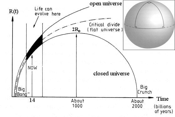
Note: For closed space the sum of the angles in a triangle would be greater than 180o; it is smaller than 180o for open space; it equals to 180o exactly for flat space.
Cosmological Constant and de Sitter Universe
It is found lately that the cosmic expansion may be accelerating. An
additional term with the cosmological constant is added to the gravitational
equation (18a) as a possible candidate for the dark energy to drive the
acceleration. It was originally introduced by Einstein to address the failure of
constructing a static universe. Thus Eq.(18a) becomes:
| (dR/dt)2 + kc2 = 8 where |
| The effect of the cosmological constant on the cosmic
expansion is summarized in Figure 10f.
|
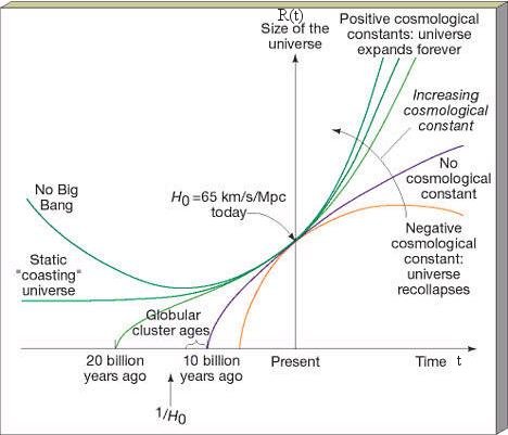
The de Sitter universe is devoid of matter energy containing only vacuum
energy. It follows that Eq.(20a) is simplified to:
(dR/dt)2 + kc2 =
![]() R2 c2
/ 3 or (dR/cdt)2 -
R2 c2
/ 3 or (dR/cdt)2 -
![]() R2 / 3 = -k
---------- (20b).
R2 / 3 = -k
---------- (20b).
For k = 0, the solution is: R(t) = R0 e![]() Ht
Ht
| where H = ( |
| For k = +1, R(t) = (c/H) cosh(Ht)
Figure 10g de Sitter Universe with k = +1
|
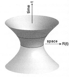
Figure 10g depicts a de Sitter universe with k = +1 from t
![]() -
-![]() to t
to t ![]() +
+![]() .
It shrinks to a minimum size of (c/H) at t = 0.
.
It shrinks to a minimum size of (c/H) at t = 0.
For k = -1, R(t) = (c/H) sinh(Ht)
![]() (c/2H) eHt as t
(c/2H) eHt as t
![]() . Its size shrinks to
zero at t = 0. There is no solution for negative t as R also becomes negative.
. Its size shrinks to
zero at t = 0. There is no solution for negative t as R also becomes negative.
All de Sitter universes expand forever exponentially. Such behaviour is similar
to the situation at the very beginning and very end of our universe, either when
energy matter had not been created or they have been diluted so much at the end.
The anti-de Sitter (AdS) universe is also described by Eq.(20b) except that ![]() is now negative.
is now negative.
For k = -1, R(t) = (c/H) sin(Ht).
where H = (-![]() /3)1/2c.
There is no solution for k = 0, and k = +1. Since a negative
/3)1/2c.
There is no solution for k = 0, and k = +1. Since a negative ![]() implies attraction, the AdS
undergoes a cycle of expansion and contraction with a time scale of
implies attraction, the AdS
undergoes a cycle of expansion and contraction with a time scale of
![]() /H (see Figure 10f).
/H (see Figure 10f).
The simple de Sitter, anti-de Sitter models suggest that for large positive
![]() , everything flies apart so
quickly that there is no chance for matter to assemble itself into sturctures
like galaxies, stars, planets, atoms or even nuclei. On the other hand, with
large negative
, everything flies apart so
quickly that there is no chance for matter to assemble itself into sturctures
like galaxies, stars, planets, atoms or even nuclei. On the other hand, with
large negative ![]() , the
expanding universe quickly turns around and terminates the evolution of life
before it can arrive at the present state. The estimated value of about 0.7x10⁻²⁹
gm/cm3 seems to be fine tuned for the existence of life. Nobody is
able to find an explanation for such coincidence yet.
, the
expanding universe quickly turns around and terminates the evolution of life
before it can arrive at the present state. The estimated value of about 0.7x10⁻²⁹
gm/cm3 seems to be fine tuned for the existence of life. Nobody is
able to find an explanation for such coincidence yet.
¶ The steady state universe requires continuous creation of matter in
order to keep the expanding universe uniform everywhere and anytime. The
refutation of the theory came with the observation that quasars were found only
at large distances. The discovery of microwave background radiation, which
indicates a much denser state further back at the time of Big Bang, finally
ruled it out completely.
Theory of Cosmic Inflation and Acceleration
| Astronomical observations over the last 20 years have indicated that the universe has experienced two periods of acceleration (see Figure 10h). The first one was a very rapid expansion soon after the Big Bang. It is usually referred to as inflation. The dark energy accelerated expansion is gentler, and has occurred only recently in the current epoch. The inflation is explained by an as yet un-identified scalar field (inflaton) undergoing a phase transition. While there are three categories of theory for the accelerated expansion: modifications to general relativity perhaps with extra dimensions, a cosmological constant, and a universal evolving scalar field. None of these offers a satisfactory explanation. |
| The followings provide a mathematical description of cosmic
inflation and expansion without invoking a detailed mechanism. Figure 10h Cosmic Inflation |
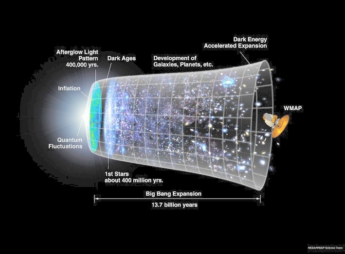
- If we assume a homogeneous and isotropic universe, with the total mass to
be constant as expressed in Eq.(18c), then Eq.(18a) can be recast into a form that shows the acceleration /
deceleration explicitly:
(d2R/dt2) / R = - 4G
/ 3 ---------- (20c)
This formula shows that the matter dominated universe in general would experience deceleration as the term on the right is always negative.
- In the presence of other forms of matter-energy, a pressure term p has to
be added into Eq.(20c):
(d2R/dt2) / R = - (4G
/ 3c2) (c2
+ 3p) --------- (20d)
- The matter-energy density
and the pressure p are usually related by the equation of state, which can be
expressed as p = wc2,
thus Eq.(20d) can be rewritten as:
(d2R/dt2) / R = - (4G
/ 3) (1 + 3w) ---------- (20e)
For relativistic matter, w = 1/3. For non-relativistic matter, w = 0. For the de Sitter universe, w = -1. The expansion of the universe will accelerate if
w < -1/3, when the right-hand side in Eq.(20e) becomes positive. The negative pressure is a characteristic of expansion under constant density as shown by a simple example. It is also known as false vacuum. In the simplest version of the inflationary paradigm a single scalar field (inflaton) dominates the energy density of the universe. To achieve the acceleration condition w < -1/3 and the observed properties of our universe, the inflation must evolve slowly such that the potential energy dominates over the kinetic energy for a sufficient part of the inflation. Figure 10i shows a theory (the old one) that doesn't work because the scalar field (the Higgs field) evolves rapidly.While the newer theory is just right creating an universe as we see it today. This scenario remains ambiguous as the precise form of the scalar field is unknown, and there is still nagging doubt about the occurrence of inflation. Figure 10i Theories of Inflation
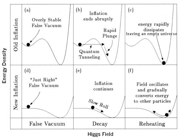
- Another way to achieve acceleration can be derived from a constant energy-matter
density term (the cosmological constant) as shown in Eq.(20a), which can be recast in the form:
(d2R/dt2) / R = - 4G
/ 3 + c2 / 3
---------- (20f)
This equation shows that at some point in the evolution of the universe the right-hand term would become positive, and the expansion would switch from deacceleration to acceleration. This condition yields the change over epoch at z = 0.72 form =
0.3, and
= 0.7. Effort to identify the cosmological constant with the vacuum energy of
the various quantum fields is not very successful. The simplest versions of
quantum theory predict far too much energy - 10120 higher than the
observed value by one estimate.
- The explanation of the current acceleration in term of an evolving scalar
field presents a tremendous hierarchy problem. The very high energy (1016
Gev) associated with the scalar field in the inflation period requires an
unreasonable amount of fine-tuning to account for the extraordinarily low
energy (10-48 Gev) of the scalar field in the current epoch.
- A different explanation was proposed by a research team in 2005, they links the dark energy acceleration to the gigantic ripples in space-time created in the epoch of inflation. In effect, it is like hobbling amid a huge undulating wave in the ocean, you don't actually see the wave (the wavelength is too long) - all you feel is the swell moving up and down.
Angular-Size Redshift Relation
| The angular-size redshift relation describes the
relationship between the angular size observed on the sky of an object of
given physical size, and the object's redshift. In elementary Euclidean
geometry the relation between angular size
In an expanding universe the distance d is a function of the redshift z: d = (c/Ho) {qoz + (qo - 1)[(1 + 2qoz)½ - 1]} / [qo2(1 + z)2] |
| where qo = (4 Figure 10j Angular-Size / Redshift
|
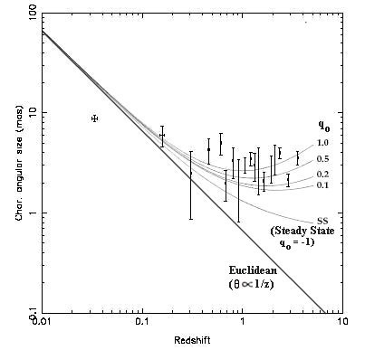
As z
![]() 0, d
0, d
![]() (c/Ho) z , and
(c/Ho) z , and
![]()
![]() 1/z
1/z
while for z ![]() , d
, d
![]() (c/Ho) / qoz,
and
(c/Ho) / qoz,
and
![]()
![]() z .
z .
| These limiting cases clearly demonstrate the curious effect
that the angular size of an object becomes larger as it is further away from
Earth. It appears to decrease with distance only for nearby objects. Figure
10k shows the infrared blobs produced by the first stars (high z objects).
It is suggested that the appearance of the puffy blobs with large angular
size is caused by the expansion of the universe with z > 1.6 as shown in
Figures 10i and 10k. Figure 10k Infrared Blobs |
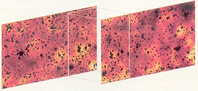 |
| In principle, the angular-size redshift relation can be used
to select the type of space for our universe. However, it is notoriously
difficult to collect reliable data in practice because the astronomical
yardstick can vary in size and in luminosity over time (the evolutionary and
selection effects). In addition, we can only measure the projections on the
celestial surface according to the orientation of the objects. All past
attempts using data from galaxies, the separation of the lobes of radio
sources, quasars, and radio galaxies produced inconclusive results. The
observational data in Figure 10l are based on selective compact radio
sources. The best fitting regression analysis gives a value of qo
|
| with ultra-compact radio sources find close match for the
model of an universe with cosmological constant,
Figure 10l Model with Cosmological Constant |
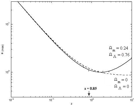
Euclidean Space
The Minkowski space-time in relativity has the signature (-,+,+,+). The
negative signature in the time component has obscure properties that make
visualization very difficult as well as creating novel features not easily
comprehensible. In many instances, the problem can be resolved partially by
substituting t ![]() it, which
transforms the Minkowski space-time to the Euclidean four-dimensional space with
signature (+,+,+,+). Sometimes, the transformation is reversed back to the
original Minkowski space-time at the end of the computation. However, some
physicists prefer to treat the Euclidean space as the ultimate reality, while
the Minkowski space-time is considered just a figment of our imagination - a
point of view not yet validated by observation. Actually, even a four-dimensional
Euclidean space is very difficult to visualize. So let us start with a three-dimensional
space as we experienced all our life.
it, which
transforms the Minkowski space-time to the Euclidean four-dimensional space with
signature (+,+,+,+). Sometimes, the transformation is reversed back to the
original Minkowski space-time at the end of the computation. However, some
physicists prefer to treat the Euclidean space as the ultimate reality, while
the Minkowski space-time is considered just a figment of our imagination - a
point of view not yet validated by observation. Actually, even a four-dimensional
Euclidean space is very difficult to visualize. So let us start with a three-dimensional
space as we experienced all our life.
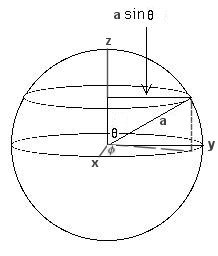 |
In 3-D Euclidean space, the formula for a sphere of radius
a located at (0,0,0) has the form: x2 + y2 + z2 = a2 with the metric ds2 = dx2 + dy2 + dz2 = a2 (d in spherical coordinates (r, |
Figure 10m 2-D Sphere
|
ds2 = a2 sin2 |
In the four-dimensional Euclidean space, the 3-D hypersphere is defined by the
formula:
x12 + x22 + x32
+ x42 = a2
and ds2 = dx12 + dx22 +
dx32 + dx42 = a2 (d![]() 2
+ sin2
2
+ sin2 ![]() d
d![]() 22)
---------- (20h).
22)
---------- (20h).
where d![]() 22
= (d
22
= (d![]() 2 + sin2
2 + sin2![]() d
d![]() 2) is an unit 2-D
sphere equivalent to d
2) is an unit 2-D
sphere equivalent to d![]() 2,
and d
2,
and d![]() 2 assumes the
role of d
2 assumes the
role of d![]() 2 in Eq.(20g).
2 in Eq.(20g).
The formulation can be generalized further to 5-D Euclidean space with the 4-D
hypersphere metric:
ds2 = a2 (d![]() 2
+ sin2
2
+ sin2![]() d
d![]() 32)
---------- (20i).
32)
---------- (20i).
where the 3-D d![]() 32
= (d
32
= (d![]() 2 + sin2
2 + sin2![]() d
d![]() 22) is
equivalent to d
22) is
equivalent to d![]() 22
in Eq.(20h).
22
in Eq.(20h).
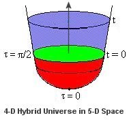 |
The no boundary proposal makes use of Eq.(20i) and suggests that at the
beginning the universe was running with
ds2 = a2 [-c2dt2 + cosh2(ct/a) d Such a hybrid universe is shown in Figure 10n. Thus, there is no singularity at the beginning of time. That particular region becomes as smooth as the North (South) pole on Earth. It is |
Figure 10n Hybrid Uni-verse |
suggested that the (red) region in Euclidean time represents
the moment of nucleation via tunneling through some sort of energy barrier
from nothing (in the form of vacuum fluctuation for example). |
The expression for d![]() 22
is just the metric on 2-D unit sphere (an ordinary sphere with radius equal to
1) in a 3-D space as shown by Eq.(20g). Similarly, d
22
is just the metric on 2-D unit sphere (an ordinary sphere with radius equal to
1) in a 3-D space as shown by Eq.(20g). Similarly, d![]() 32
is the metric on 3-D unit hypersphere in a 4-D space. In general, d
32
is the metric on 3-D unit hypersphere in a 4-D space. In general, d![]() n2
denotes the metric on n-dimensional hypersphere in a (n+1)-dimensional space. It
is always possible to create n-dimensional hypersphere and other geometrical
shapes in a (n+1) dimensional space including the Euclidean and many others. For
example, a 4-D hypersphere can be embedded in a 5-D anti-de Sitter space with
metric in the following form:
n2
denotes the metric on n-dimensional hypersphere in a (n+1)-dimensional space. It
is always possible to create n-dimensional hypersphere and other geometrical
shapes in a (n+1) dimensional space including the Euclidean and many others. For
example, a 4-D hypersphere can be embedded in a 5-D anti-de Sitter space with
metric in the following form:
ds2 = d![]() 2
+ sinh2(
2
+ sinh2(![]() /l) d
/l) d![]() 42
---------- (20j).
42
---------- (20j).
where l = (-![]() /3)-1/2,
and d
/3)-1/2,
and d![]() 42
= a2(d
42
= a2(d![]() 2 +
sin2
2 +
sin2![]() d
d![]() 32)
is the 4-D hypersphere.
32)
is the 4-D hypersphere.
This 5-D AdS space has been used to apply the holographic principle to physical theories or objects (such as superstring theory or black hole) by
encoding them from such 5-D space to a 4-D hypersphere.
Five Dimensional Space-time
| It is found that when 4-dimensional theory is formulated in a 5-dimensional space-time, novel features emerge as the theory is reduced back to 4-D. The Kaluza-Klein theory introduced in the 1920s is the most famous example, which unifies the theories of gravitation and electromagnetism. The technique of compactification to hide the extra-dimension is now used extensively in the superstring theory. It is from the process of compactification that produces various particle properties. |
| Figure 10o 5-D Space-time
|
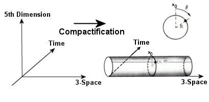
Let us first consider the simple example of the massless Klein-Gordon
equation in quantum field theory. In 4-D space-time, this equation has the form:
![]()
![]() (x
(x![]() )
= 0 ---------- (20k)
)
= 0 ---------- (20k)
where
![]()
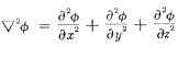 ,
and the index
,
and the index ![]() runs from 1 to 4
(with the 4th index identified to the time component).
runs from 1 to 4
(with the 4th index identified to the time component).
The extension to 5-D space-time can be accomplished very easy by including an
extra variable x0 in the formulation, and let
![]() runs from 0 to 4. Then Eq.(20k)
becomes:
runs from 0 to 4. Then Eq.(20k)
becomes:
![]() 5
5![]() (x
(x![]() ,x0)
= 0 ---------- (20l)
,x0)
= 0 ---------- (20l)
where an additional second partial derivative in x0 is inserted into
the equation. Such 5-D space-time is shown in the left of Figure 10o. Since the
real world is three dimensional in spatial coordinates, we can consider the
unobservable extra dimension to curl-up into very small circle (at every point
in the 3-D space) as shown in the right of Figure 10o. Under this circumstance,
the extra dimension would become periodic with x0 = x0 + 2![]() R,
where R is the radius of this space. Consequently, the scalar field can be
expressed in terms of periodic functions:
R,
where R is the radius of this space. Consequently, the scalar field can be
expressed in terms of periodic functions:
![]() (x
(x![]() ,x0)
=
,x0)
= ![]() (x
(x![]() )
eip0x0
)
eip0x0
where p0 = n / R to satisfy the periodic condition, and n is an
arbitrary integer. Thus, Eq.(20l) can be reduced to the form:
![]() 5
5![]() =
=
![]()
![]() - (n / R)2
- (n / R)2![]() = 0
---------- (20m)
= 0
---------- (20m)
which is just the 4-D space-time Klein Gordon Equation with effective mass = (n
/ R). This is a very simple example of Kaluza-Klein tower (also known as KK
particles, KK modes), which in effect is the energy of the standing waves in the
extra compactified dimension (Figure 10p). In the n = 0 mode, the KK particle
will be indistinguishable from the known particles. The lightest KK particle
corresponds to n = 1; it would have the same charge as the known particles but
different mass.
| If experimenters discover new heavy particles with the same charges as familiar ones and masses that are similar to one another, those particles will be strong evidence of extra dimensions. If such particles also occur at regular intervals of mass, it would very likely mean that a simple curled-up dimension has been discovered. But more complicated extra-dimensional geometries will yield more complicated patterns of masses. If enough such particles are discovered, the KK particles would then reveal not only the existence of extra dimensions, but also the their sizes and shapes. Since no KK particle has been detected so far, it seems to indicate that the size of the curled-up dimension could be very small. |
| In unit of ev, the mass of the KK tower Mn =
(n/R) x 1.2 x 10⁻⁴ ev. Thus, the new LHC collider (to be
operational in 2007) with available energy up to 14 Tev can probe the curled-up
dimension down to the size of about 10-17 cm. Figure 10p KK Tower
|
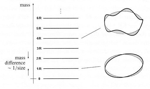
- The compactification of a dimension creates a quantization of the momentum corresponding to the compactified coordinate. The momentum is labeled by integers.
- The mass spectrum in the space-time dimensions that are not compactified is shifted by an effective mass term coming from the compactified dimension.
- The radius of the compactified dimension can be totally arbitrary as long as it can hide that dimension from observation.
- In general the components with
 from 1 to 4 will recover the
original theory with additional term. The
= 0 component will generate
some kind of physical property. In some other theories when there are cross
terms between the = 1, ...,4
and the = 0 components, other
theories will emerge from the reduction.
from 1 to 4 will recover the
original theory with additional term. The
= 0 component will generate
some kind of physical property. In some other theories when there are cross
terms between the = 1, ...,4
and the = 0 components, other
theories will emerge from the reduction.
Several conclusions can be drawn from this simple example:
Similarly in the Kaluza-Klein theory, the gravitational field equation in 5-D
space-time can be reduced to:
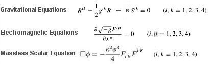
- The extra dimension is not curl-up and satifies the periodic condition. It is proposed instead that gik should not depend on x0, which implies g00 is a constant.
- The reduction of the (
 ,
) (from 1 to 4), (0,
), and (0, 0) components of
the curvature tensor respectively generates the gravitational, electromagnetic,
and scalar fields.
,
) (from 1 to 4), (0,
), and (0, 0) components of
the curvature tensor respectively generates the gravitational, electromagnetic,
and scalar fields. - The reduced equations for gravity is similar to the original gravitational
field equations in Eq.(12a). The additional term
 is the electromagnetic stress-energy tensor, and k ~ g00 is
the gravitational constant.
is the electromagnetic stress-energy tensor, and k ~ g00 is
the gravitational constant. - The electromagnetic equations are modified by a factor of (-g)1/2,
where g is the determinant formed from gik.
F
= g0,
- g0,
is the electromagnetic anti-symmetric tensor defined in the original equations. Indices separated by a comma will denote differentiation with respect to the
corresponding coordinate. - The massless scalar field is called radion or dilaton. It can be interpreted as the length or size of the fifth dimension as a function of the usual four dimensions of space-time. In string theory, the dilaton always appears together with gravity.
- The equation of motion in the reduced 4-D space-time takes the form:
where0 is the mass
density. The interaction terms involve the gravitational field interacting
with the energy-momentum density, and the electromagnetic field interacting
with the charge-current density.
Some comments on the Kaluza-Klein theory:
| Nowadays, we know that electromagnetism and gravity are far from being the whole story. A satisfactory unified theory must accommodate a good deal more like the weak and strong interactions. In fact, five dimensions are not enough; we might just manage with ten (such as in the string theory). The Kaluza-Klein method has been generalized to Yang-Mills theory in (4+N)-dimensional spac-time. If supersymmetry is added to the formulation, the new components of the super curvature tensor emerge as |
| quarks and leptons. Such formulism is called supergravity.
The decomposition is illustrated in a much simplified form in Figure 10q.
Figure 10q Supergravity
|
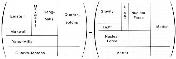
It seems that everything is there. The most serious problem with quantum
Kaluza-Klein theory is that it is non-renormalizable; and the fact that certain
particles are missing in this picture eventually forces physicists to develop a
more powerful formalism: the superstring theory.
But the central theme of Kaluza-Klein theory remains: the physical laws depend
on the geometry of hidden extra dimensions.
Quantum and atom - Quantum Worlds
Hiçbir yazı/ resim izinsiz olarak kullanılamaz!! Telif hakları uyarınca bu bir suçtur..! Tüm hakları Çetin BAL' a aittir. Kaynak gösterilmek şartıyla siteden alıntı yapılabilir.
The Time Machine Project © 2005 Cetin BAL - GSM:+90 05366063183 -Turkiye/Denizli
Ana Sayfa /index /Roket bilimi /![]() E-Mail /CetinBAL/Quantum Teleportation-2
E-Mail /CetinBAL/Quantum Teleportation-2
Time Travel Technology /Ziyaretçi Defteri /UFO Technology/Duyuru