Time Travel Research Center © 2005 Cetin BAL - GSM:+90 05366063183 - Turkey / Denizli
Deviation of Light near the Sun
in General Relativity
Christian Magnan
The deviation of light rays near the Sun is one of the most dramatic predictions of general relativity and the verification of this effect by Eddington in 1919 brought a spectacular confirmation of Einstein's theory. But it is quite difficult to provide the reader with the details of the calculation as there is no simple way to do it. In fact, to get the result it is necessary to dive into the full theory of general relativity. Here is a good opportunity to discover this theory while illustrating it on an example!
The derivation of the equations given here closely follows the presentation of Edwin F. Taylor and John Archibald Wheeler in their delightful work "Exploring Black Holes, Introduction to General Relativity" (Addison Wesley Longman, 2000).
In Special Relativity space-time curvature is thought to be
responsible for gravitational lensing.
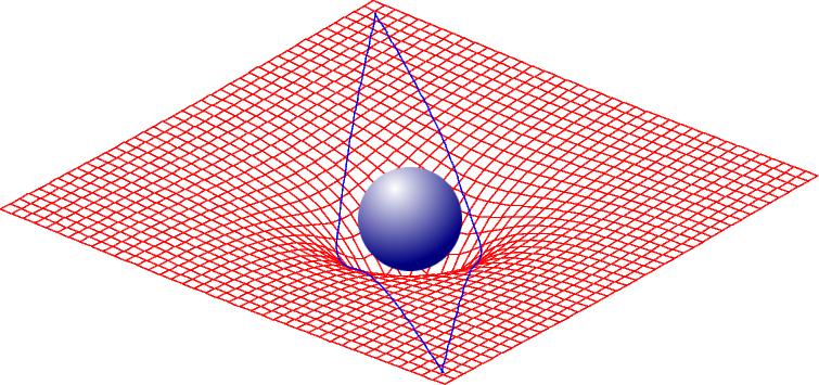
In this model light travels in a straight path through space-time. Space-time
is thought to be warped or curved by the presence of matter. As light
travels near a massive object its trajectory will be bent as a result of
the curved space-time.
It is impossible a curved space-time will produce the effects we see in
gravitational lensing. According to special relativity as light
approaches a massive object its space-time curves which only appears to
bend the light. But as the light reaches the other side of the massive
object its path through the curvature of space-time would be exactly the
opposite as its approach resulting in the light bending back to its
original direction. If special relativity were observationally true we
would not see any gravitational lensing what-so-ever.
There has to be another explanation for gravitational lensing because
the one we have is incorrect.
-
Principle of the calculation
Metrics for curved spacetime around a massive object
The equations of a geodesic
Energy of the particle
Angular momentum of the particle
Computing the orbit
The trajectory of light
Determination of the deflection angle
Approximations and integration
About this document...
Principle of the calculation
Whereas the qualitative aspect and the historical impact of the phenomenon of light bending near the Sun are described in many places, the calculation of the angle of deviation is rarely given. This page is dedicated to this numerical exercise.
General relativity teaches us that by propagating into space a photon follows what is called a "geodesic" of spacetime. Thus we have to examine the following points:
- what is a "geodesic"?
- which equations govern a geodesic?
- find the solutions of those equations and thus discover the trajectory of light through space
- compute the angle between the initial and final directions of light.
Metrics for curved spacetime around a massive object
Newtonian mechanics describes the motion of a particle in an absolute
space with respect to an absolute time. The position of the moving object is
located by its coordinates with respect to some frame of reference and is
given as a function of time
![]() . General
relativity affirms that there exists no absolute time ant that time cannot
be dissociated from space. The theory bases its reasoning on events,
each event being characterized by a point M (where it happens!) and a time
. General
relativity affirms that there exists no absolute time ant that time cannot
be dissociated from space. The theory bases its reasoning on events,
each event being characterized by a point M (where it happens!) and a time
![]() (when it
happens!). The events attached to a moving particle constitute what is
called a worldline.
(when it
happens!). The events attached to a moving particle constitute what is
called a worldline.
Let us consider for example a spaceship moving freely through space,
which means that all his motors are turned off. Let us imagine that regular
flashes are emitted in accordance with a clock located inside the rocket and
beating the time. The time interval between two successive flashes will be
denoted by ![]() (this
quantity is thus measured with respect to the proper time of the spaceship).
Think now of another frame of reference as constituted by an ensemble of
space beacons, also free from acceleration, at constant mutual distances
from one another (each free beacon stays at the same distance from its
neighbours). Every signal bears the indication of its position in space (for
instance by showing its distance from some origin) and holds its own clock.
The clocks of this second frame are synchronized between them. Then in that
frame the interval between two flashes (i.e. two events) is characterized by
two numbers: the space interval
(this
quantity is thus measured with respect to the proper time of the spaceship).
Think now of another frame of reference as constituted by an ensemble of
space beacons, also free from acceleration, at constant mutual distances
from one another (each free beacon stays at the same distance from its
neighbours). Every signal bears the indication of its position in space (for
instance by showing its distance from some origin) and holds its own clock.
The clocks of this second frame are synchronized between them. Then in that
frame the interval between two flashes (i.e. two events) is characterized by
two numbers: the space interval
![]() and the time
interval
and the time
interval ![]() . To
determine those two quantities it suffices to record which beacon faces
Flash #1 and which beacon faces Flash #2 while noting the times of those
events.
. To
determine those two quantities it suffices to record which beacon faces
Flash #1 and which beacon faces Flash #2 while noting the times of those
events.
Special relativity is based on the following principle. The proper time
interval ![]() between Event #1 et Event #2 is given by the formula
between Event #1 et Event #2 is given by the formula
|
|
(1) |
and this quantity does not depend on the frame in which it is evaluated.
In other words all observers agree on the value of
![]() computed by
Formula (1), although the values of
computed by
Formula (1), although the values of
![]() and
and
![]() differ from
one system of reference to another.
differ from
one system of reference to another.
Be careful: unless otherwise indicated, distances will be measured in
units of time, as is often done in astronomy. We have chosen to do so in
writing Equation (1). On the contrary if distances s are expressed in
conventional units, for instance in centimeters, then one should pass from
the latter to our distance s expressed in seconds via the formula
![]() cm/s.
(Expressing distances and times with the same unit would amount to taking
the speed of light equal to unity.)
cm/s.
(Expressing distances and times with the same unit would amount to taking
the speed of light equal to unity.)
In general relativity the property of invariance of the proper interval
with respect to a change of the coordinates remains valid but only locally,
i.e. under the condition of staying in a sufficiently small region of
spacetime (its size depends on the accuracy of the measurements). The main
novelty concerns the expression of the proper time as given by Formula (1).
The coefficients entering this formula depend now on the point of spacetime
under consideration and the resulting expression takes the name of
metrics. In fact the whole structure of spacetime, and especially its
curvature, is included in the local expression of
![]() and in the form of its coefficients.
and in the form of its coefficients.
We are interested here in the structure of spacetime around the sun. In
order to describe the physics locally we consider two nearby events
separated by infinitesimal amounts of the time and space coordinates
![]() ,
,
![]() ,
,
![]() and
and
![]() .
If space were flat, the metrics would have the form
.
If space were flat, the metrics would have the form
![]()
which is usually written (and a little sloppily) by convention as
|
|
(2) |
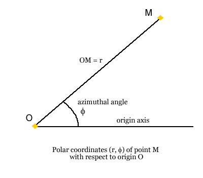
By working in spherical coordinates, in a plane containing the center of the sun (this choice removes one spatial coordinate), that formula becomes
![]()
where r denotes the distance to the center and
![]() an azimutal angle in the plane of the orbit (see the figure below).
an azimutal angle in the plane of the orbit (see the figure below).
But spacetime around a center of attraction of mass
![]() (for instance a black hole or the vicinity of the sun) is not flat. It is
characterized by the Schwarzschild metric
(for instance a black hole or the vicinity of the sun) is not flat. It is
characterized by the Schwarzschild metric
|
|
(3) |
The story is really fantastic: the whole structure of spacetime is embodied in this "simple" formula (3).Even the famous black hole lurks behind those apparently innocuous symbols.
One question: in which units is expressed the mass
![]() in that formula? It is seen that
in that formula? It is seen that
![]() has the dimension of a length, a quantity that we measure here in seconds.
Therefore
has the dimension of a length, a quantity that we measure here in seconds.
Therefore
![]() will also be measured in seconds. The formula allowing to transform grams in
seconds is
will also be measured in seconds. The formula allowing to transform grams in
seconds is
![]()
where
![]() .
.
The equations of a geodesic
The metric, that is (exactly) the formula expressing at a givent point of
spacetime the temporal interval between two nearby events, reveals the
presence of curvature as soon as the expression deviates from Formula (2)
corresponding to flat euclidian space. That metric will allow us to find the
properties of the motion of a test particle free from acceleration. Actually
both special and general relativity teach us that between two given events
![]() and
and
![]() a freely moving body follows the path for which the time interval
a freely moving body follows the path for which the time interval
![]() is maximum. Equivalently one can say that a freely moving particle follows a
geodesic of spacetime as a geodesic is precisely defined by this property of
maximazing the time interval.
is maximum. Equivalently one can say that a freely moving particle follows a
geodesic of spacetime as a geodesic is precisely defined by this property of
maximazing the time interval.
Definition of a geodesic: the geodesic between two eventsand
is the wordline for which the interval of proper time between
That property of maximazing the proper time will allow us to derive the equations of a geodesic. It will also yield the expressions of the energy and angular momentum of a particle in orbit around the center of attraction.
Energy of the particle
Let us apply the principle of maximisation of the proper time interval in
the following manner. Suppose that a free spatial ship (whose rockets are
turned off) falls radially, therefore along a straight path, towards the
central attractive mass. Imagine that three successive flashes, with nearby
time and space coordinates, are emitted inside the spaceship. We observe
those three events in some external frame. In that latter frame the event
![]() consists in the emission of a flash at time
consists in the emission of a flash at time
![]() when the spatial engine is located at radius
when the spatial engine is located at radius
![]() .
The flash
.
The flash
![]() is emitted at time
is emitted at time
![]() when the cabin is at radius
when the cabin is at radius
![]() .
The flash
.
The flash
![]() is emitted at time
is emitted at time
![]() when the cabin is at radius
when the cabin is at radius
![]() .
The quantity
.
The quantity
![]() is assumed to be small. We then assume that we vary the intermediate
coordinates of
is assumed to be small. We then assume that we vary the intermediate
coordinates of
![]() .
The principle of maximal aging says that the geodesic starting from
.
The principle of maximal aging says that the geodesic starting from
![]() and ending at
and ending at
![]() will pass through Event
will pass through Event
![]() such that the proper time interval
such that the proper time interval
|
|
(4) |
is maximum. Here
![]() measures the interval over the first spacetime segment
measures the interval over the first spacetime segment
![]() ,
which connects
,
which connects
![]() to
to
![]() and
and
![]() measures the time interval over the second segment
measures the time interval over the second segment
![]() ,
which connects
,
which connects
![]() to
to
![]() .
.
In order to avoid varying all quantities at the same time, we assume in
this experiment that the locations of the radii
![]() ,
,
![]() and
and
![]() are fixed and that only the time
are fixed and that only the time
![]() ,
at which the second flash is emitted, is allowed to change. According to
Formula (3) the interval of proper time over the first segment
,
at which the second flash is emitted, is allowed to change. According to
Formula (3) the interval of proper time over the first segment
![]() is given by its square
is given by its square
|
|
(5) |
from which we deduce
|
|
(6) |
The lapse of time over Segment
![]() between the events
between the events
![]() and
and
![]() is
is
![]() ,
and therefore the proper time duration
,
and therefore the proper time duration
![]() is given by
is given by
|
|
(7) |
from which we deduce
|
|
(8) |
To make the total time interval
![]() maximum with respect to a variation
maximum with respect to a variation
![]() of the time
of the time
![]() ,
we write
,
we write
|
|
(9) |
Deducing
![]() and
and
![]() from Equations (6) and (8) and letting quite naturally
from Equations (6) and (8) and letting quite naturally
![]() and
and
![]() ,
we easily get
,
we easily get
|
|
(10) |
The left side of that equation depends only on parameters characterizing
the first segment A (which connects
![]() to
to
![]() ).
The right side depends only on parameters related to the second segment B (which
connects
).
The right side depends only on parameters related to the second segment B (which
connects
![]() to
to
![]() ).
).
We have discovered in Equation (10) a quantity that is the same for both segment. This quantity is thus a constant of the motion for the free particle under consideration. For good physical reasons (especially to recover the formulae of special relativity), one is led to identify that constant of motion as the ratio of the energy of the particle to its mass. We write this very important result under the form
|
|
(11) |
an expression in which we have returned to the differential notation for
the intervals
![]() and
and
![]() .
.
Incidentally we may notice that with the units we have chosen, energy
![]() and mass
and mass
![]() are expressed in the same unit (for instance the centimeter).
are expressed in the same unit (for instance the centimeter).
Angular momentum of the particle
We have applied the principle of maximazing the proper time interval by
varying the time of the intermediate event E2. We
now perform the same operation but this time we vary the angle
![]() of that intermediate event. We recall that
of that intermediate event. We recall that
![]() measures the direction of the moving particle with respect to some direction
chosen as the origin. We call it the azimuth.
measures the direction of the moving particle with respect to some direction
chosen as the origin. We call it the azimuth.
We consider again three events consisting in the emission of flashes
inside a spaceship floating freely in space. The first segment
![]() connects Event
connects Event
![]() to Event
to Event
![]() .
The second segment
.
The second segment
![]() connects
connects
![]() to
to
![]() .
The azimutal angle of the first event is fixed at
.
The azimutal angle of the first event is fixed at
![]() .
The angle of the last one is fixed at
.
The angle of the last one is fixed at
![]() .
The intermediate azimuth is taken as the variable
.
The intermediate azimuth is taken as the variable
![]() .
Again in order not to vary everything at the same time, we assume that the
radius
.
Again in order not to vary everything at the same time, we assume that the
radius
![]() at which the second flash is emitted stays constant.
at which the second flash is emitted stays constant.
We follow the same chain of reasoning as in the previous section. From
the metric (3), the time interval
![]() over the first segment is given by its square
over the first segment is given by its square
|
|
(12) |
and the interval
![]() over the second by
over the second by
|
|
(13) |
from which we get
|
|
|
|
(14) |
|
|
|
|
(15) |
By writing
![]() one easily obtains, similarly to Formula (10)
one easily obtains, similarly to Formula (10)
|
|
(16) |
after having written quite naturally
![]() and
and
![]() .
The left side, which contains only terms that are specific to the first
segment, is equal to the right side, which contains only terms relative to
the second segment. We thus exhibit another constant of motion, namely
.
The left side, which contains only terms that are specific to the first
segment, is equal to the right side, which contains only terms relative to
the second segment. We thus exhibit another constant of motion, namely
![]() (by shifting back to the differential notation), a quantity that turns out
to be identified with the ratio of the angular momentum
(by shifting back to the differential notation), a quantity that turns out
to be identified with the ratio of the angular momentum
![]() of the particle to its mass
of the particle to its mass
![]() ,
which we write as
,
which we write as
|
|
(17) |
Computing the orbit
Technically speaking in order to determine the trajectory of a moving
body free from acceleration we apply the following strategy. Knowing the
energy
![]() and the angular momentum
and the angular momentum
![]() of the particle of mass
of the particle of mass
![]() (
(![]() and
and
![]() depend on the initial conditions) we can follow the position of that
particle by computing the increments of its spacetime coordinates
depend on the initial conditions) we can follow the position of that
particle by computing the increments of its spacetime coordinates
![]() ,
,
![]() and
and
![]() as the proper time
as the proper time
![]() itself advances. Algebraically for each increment
itself advances. Algebraically for each increment
![]() of the proper time we compute (or the computer calculates) the corresponding
increments
of the proper time we compute (or the computer calculates) the corresponding
increments
![]() ,
,
![]() and
and
![]() of the coordinate of the mobile body. The squares of the increments
of the coordinate of the mobile body. The squares of the increments
![]() and
and
![]() are extracted from Equations (11) and (17) in the following form:
are extracted from Equations (11) and (17) in the following form:
|
|
|
|
(18) |
|
|
|
|
(19) |
We notice that the expression of
![]() is missing. We get it by transporting the values of
is missing. We get it by transporting the values of
![]() and
and
![]() into the metric equation (3) and solving it for
into the metric equation (3) and solving it for
![]() .
This yields
.
This yields
|
|
(20) |
By dividing both sides of Equations (20) and (19) we directly arrive to
the equation of the orbit in polar coordinates as
|
|
(21) |
The trajectory of light
The preceding treatment is apparently not relevant to the case of a
photon. In fact the calculation of the trajectory was done by incrementing
the proper time but this latter concept has no meaning for a photon since
the interval between two events that are located on the wordline of a photon
is always equal to zero (as at light velocity
![]() ,
the interval
,
the interval
![]() vanishes).
vanishes).
Nevertheless it happens that by letting the mass of the particle tend
towards zero, one arrives at the right results. Thus for
![]() our equation (21) takes the form
our equation (21) takes the form
|
|
(22) |
That equation will allow us to determine the deviation of ligth rays passing near the sun.
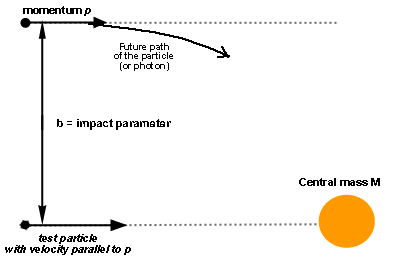
It is necessary to specify the parameters found in the formulae. First
the angular momentum of the moving particle at infinity is equal by
definition to the product of its linear momentum
![]() by what is called the impact parameter
by what is called the impact parameter
![]() ,
which represents the distance between the center of attraction (the sun in
the present case) and the initial direction of the velocity of the particle
(see the figure).
,
which represents the distance between the center of attraction (the sun in
the present case) and the initial direction of the velocity of the particle
(see the figure).
In other words
|
|
(23) |
In addition it is known that the momentum
![]() of a photon is equal to its energy
of a photon is equal to its energy
![]() (with the units that were chosen). It results at once from this formula that
(with the units that were chosen). It results at once from this formula that
|
|
(24) |
If the ratio
![]() is equal to the impact parameter
is equal to the impact parameter
![]() Equation (22) writes as
Equation (22) writes as
|
|
(25) |
Determination of the deflection angle
Formula (25) will allow us to determine the change in the direction of a
light pulse caused by the gravitational field of the sun. To achieve this
aim we have to sum up the successive infinitesimal increments
![]() of the azimuthal angle
of the azimuthal angle
![]() along the path. This means that we have to carry out the integration of
along the path. This means that we have to carry out the integration of
![]() when r varies from the minimum distance denoted
when r varies from the minimum distance denoted
![]() (
(![]() is the radius of the sun if the light ray grazes its surface). We should
still multiply that quantity par 2 to account for both symmetrical "legs" of
the trajectory (the photon first approaches the Sun then recedes from it).
is the radius of the sun if the light ray grazes its surface). We should
still multiply that quantity par 2 to account for both symmetrical "legs" of
the trajectory (the photon first approaches the Sun then recedes from it).
It is necessary to stipulate a further point, namely the relation
existing between the two quantities
![]() and
and
![]() that we have introduced and that are not independent. The point
that we have introduced and that are not independent. The point
![]() corresponds to the place where the light photon is closest to the sun. There
the photon moves tangentially. Since at that point there is no radial
component, we can write that the derivative
corresponds to the place where the light photon is closest to the sun. There
the photon moves tangentially. Since at that point there is no radial
component, we can write that the derivative
![]() vanishes. It suffices to take the element
vanishes. It suffices to take the element
![]() from Equation (25) to find immediately
from Equation (25) to find immediately
|
|
(26) |
so that this same equation (25) becomes
|
|
(27) |
The form of the expression dictates to us to pose
![]()
where
![]() varies between 1 and 0. The last equation (27) then becomes
varies between 1 and 0. The last equation (27) then becomes
|
|
|
|
|
| or | |||
|
|
|
|
(28) |
Consequently the infinitesimal variation
![]() of the azimuth is given in terms of the variation
of the azimuth is given in terms of the variation
![]() of
of
![]() by
by
|
|
|
|
|
|
|
![$\displaystyle \frac{(1-u^2)^{-1/2} du }{[1 - (2M/R)(1-u^3)(1 - u^2)^{-1}]^{1/2}}$](../FJ/jimg100.gif) |
(29) |
The presence of the term
![]() in Expression (29) encourages us to make the change of variable
in Expression (29) encourages us to make the change of variable
![]()
which leads to
|
|
(30) |
By observing that
![]()
we end up with the final equation of the trajectory under the form
|
|
(31) |
with
![]()
It is interesting to emphasize that so far there have been no approximation. This is quite rewarding.
Approximations and integration
The small value of the term
![]() will allow us to make an approximation and in this way will make us able to
complete the integration. In conventional units the mass of the sun is
will allow us to make an approximation and in this way will make us able to
complete the integration. In conventional units the mass of the sun is
![]() grams
and its radius is
grams
and its radius is
![]() centimeters.
By using the factor
centimeters.
By using the factor
![]() cm/g
which makes it possible to transform grams into centimeters, we get
cm/g
which makes it possible to transform grams into centimeters, we get
![]()
In Equation (31) we can thus use the classical approximation
![]() to arrive at
to arrive at
|
|
(32) |
Therefore the total variation of the azimuth
![]() along the path of the photon is
along the path of the photon is
|
|
|
![$\displaystyle 2 \int_0^{\pi/2} \left[1 + (M/R)\left( \cos\alpha + \frac{1}{1+\cos\alpha}\right)\right] d\alpha$](../FJ/jimg115.gif) |
(33) |
|
|
![$\displaystyle 2 \left[ \alpha + \frac{M}{R}\left(\sin\alpha + \tan\frac{\alpha}{2}\right) \right]_0^1$](../FJ/jimg116.gif) |
(34) | |
|
|
|
(35) |
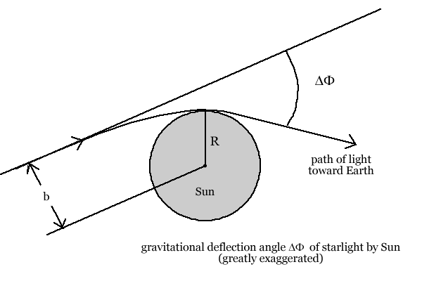
The first term
![]() gives the total change in the azimuthal angle of the photon where there is
no Sun present, since in that case the photon follows a straight path. But
the second term gives the additional angle of deflection
gives the total change in the azimuthal angle of the photon where there is
no Sun present, since in that case the photon follows a straight path. But
the second term gives the additional angle of deflection
![]() with respect to this straight line (see the figure)
with respect to this straight line (see the figure)
|
|
|
|
(36) |
| or in conventional units | |||
|
|
|
|
(37) |
Numerically at the surface of the sun (with the values of the mass and
the radius given above) one finds
![]() radian,
or ( knowing that
radian,
or ( knowing that
![]() radians equal 180 degrees and that there are 60 minutes of arc in one degree
and 60 seconds of arc in one minute of arc)
radians equal 180 degrees and that there are 60 minutes of arc in one degree
and 60 seconds of arc in one minute of arc)
![]()
Hiçbir yazı/ resim izinsiz olarak kullanılamaz!! Telif hakları uyarınca bu bir suçtur..! Tüm hakları Çetin BAL' a aittir. Kaynak gösterilmek şartıyla siteden alıntı yapılabilir.
The Time Machine Project © 2005 Cetin BAL - GSM:+90 05366063183 -Turkiye/Denizli
Ana Sayfa /
index /Roket bilimi /![]() E-Mail /CetinBAL/Quantum Teleportation-2
E-Mail /CetinBAL/Quantum Teleportation-2
Time Travel Technology /Ziyaretçi Defteri /UFO Technology/Duyuru